

If I know a lot about elliptic curves then surely I can wiggle myself into a small fortune.
Here are some free GPU credits from Runpod.
LeetArxiv is Leetcode for implementing Arxiv and other research papers.
This is Chapter 6 in our upcoming book: A Programmer’s Attempt at Hacking Satoshi’s Billion Dollar Wallet.
Available Chapters
Chapter 1 : A Programmer’s Introduction to Elliptic Curves.
Chapter 2 : What Every Programmer Needs To Know About Conic Sections (To Attack Bitcoin)
Chapter 3 : The Discrete Logarithm Problem and the Index Calculus Solution.
Chapter 4: Smart Attack on Elliptic Curves.
Chapter 5: The US Government Hid a Mathematical Backdoor in another Elliptic Curve.
Chapter 6: Hacking Dormant Bitcoin Wallets in C coding guide.
Chapter 7: Pollard’s Rho and Kangaroo Collision Searching
1.0 Introduction
Our previous chapter demonstrated a step-by-step approach to bruteforcing a dormant bitcoin wallet. This chapter illustrates practical compiler optimizations to the elliptic curve library we wrote earlier:

1.1 Quick Recap
Bitcoin wallets use an elliptic curve defined over 𝔽p called secp256k11. The curve exists in a finite field modulo:

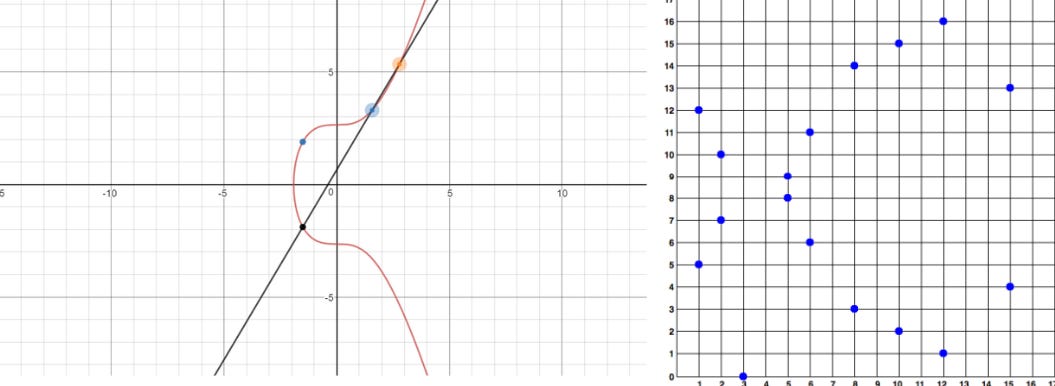
The actual curve is y2 = x3 + 7 with the visual representation:
secp256k1 is defined over a large prime number. This makes the curve secure from brutefore attacks. However, if one solves the Elliptic Curve Discrete Logarithm problem, then one can access Satoshi’s billion-dollar wallet.
Let E be an elliptic curve defined over a finite field 𝔽p and let S, T ∈ E(𝔽p). The Elliptic Curve Discrete Logarithm Problem (ECDLP) is the challenge of finding an integer m satisfying (Silverman, 2007):2

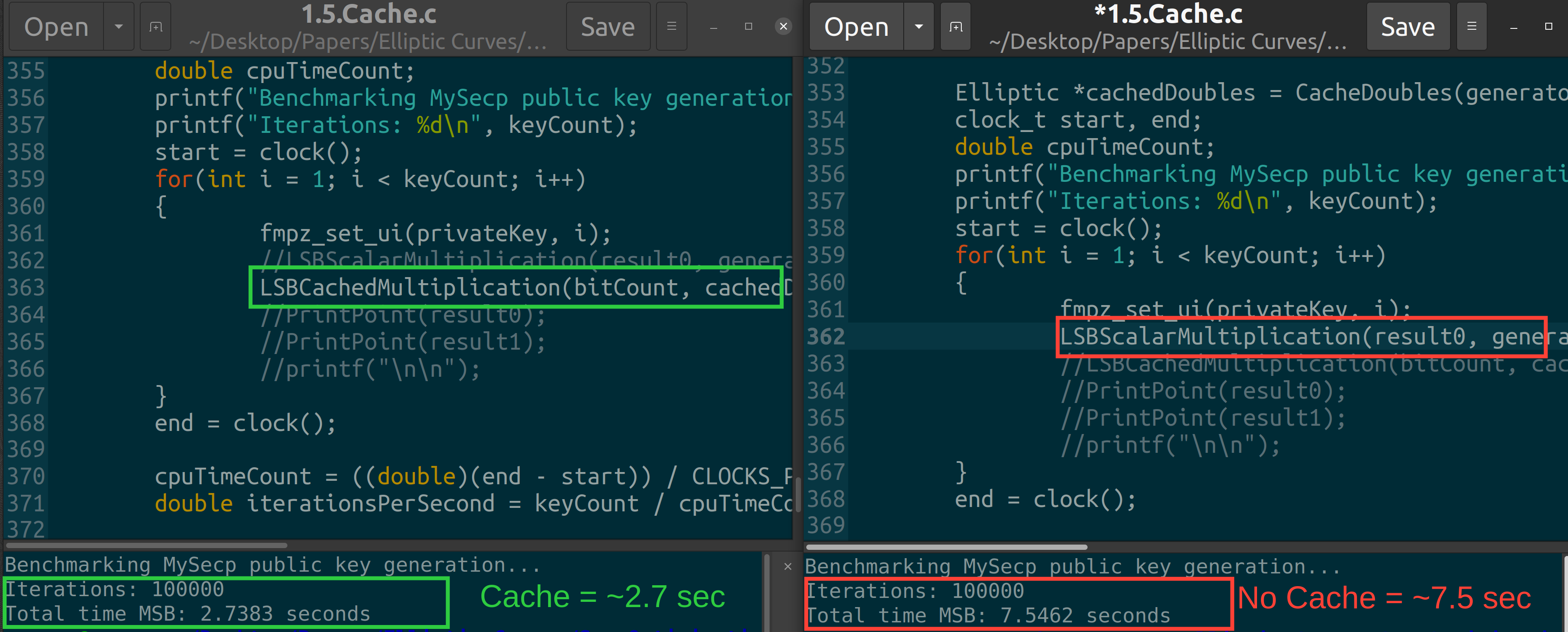
We wrote here an elliptic curve arithmetic library called MySecp. The library calculates 100,000 private keys on CPU in 7.5417 seconds. This is abysmal. Libsecp256 on the other hand, takes ~2.9 seconds to find 100,000 private keys.
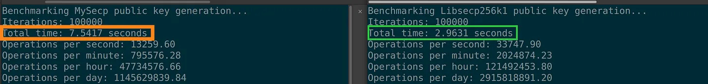
It will take ~352 million years to navigate the 67-bit bitcoin puzzle #130 search space using the MySecp library .
(2^67 keys) / (13259 keys/sec) = 352,675,523 CPU years1.2 Establishing our Goal

We aim to construct keys in less than 352 million years. Our approach is two-fold:
Either we reduce the key search space by a lot.
But, binary is logarithmic. I don’t know where to even start.
Or, we profoundly increase the number of keys calculated per second.
This is much more practical.
1.3 List of Optimizations
Bitcoin’s secp256k1 curve is pretty quirky. We optimize for bruteforce key calculation like this:
Rewriting Scalar Multiplication
We go from MSB to LSB double and add.
Precalculate our generators to get rid of doubling.
Find an integer generator for the curve’s points.
Reduce overall additions in favor of point doublings.
Writing a customised Pollard Rho/Kangaroo.
This version of Rho/Kangaroo is more stable than the one we wrote in Chapter 6.
2.0 Rewriting Scalar Multiplication
Scalar multiplication involves multiplying our generator point by the public key modulo our prime number. The double-and-add algorithm is used to achieve scalar multiplication on elliptic curves and we covered it here.
2.1 From MSB to LSB double and add.
However, there are two different ways to implement the double and add algorithm on an elliptic curve. Either LSB → MSB or MSB → LSB.
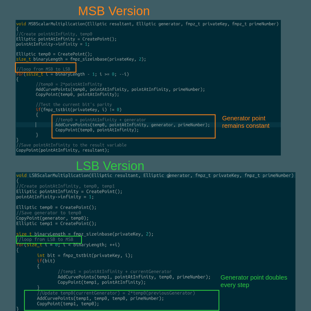
So we can start from either side of the binary string and get the same result:
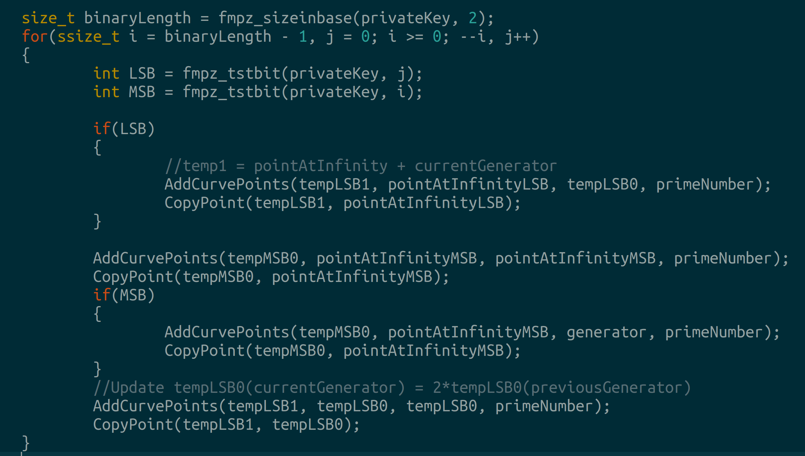
This means, we can combine the LSB and MSB approach to meet in the middle (if we want):
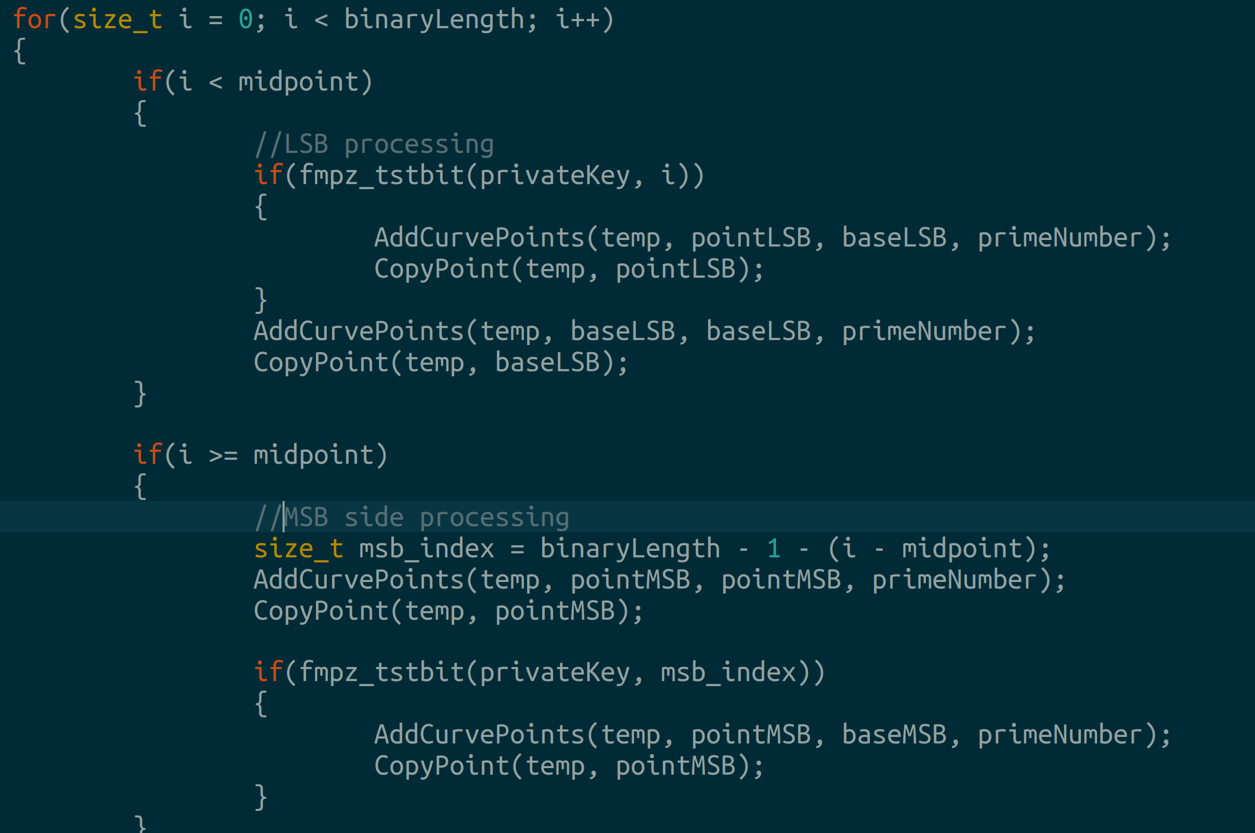
That is we can precompute a midpoint, then add LSB and MSB sums to yield a single result.
2.2 Precalculating Generators
The LSB approach suggests we can precalculate generators that are powers of 2 and sum them to get our desired key.
Let’s write a function to create a generator lookup table:
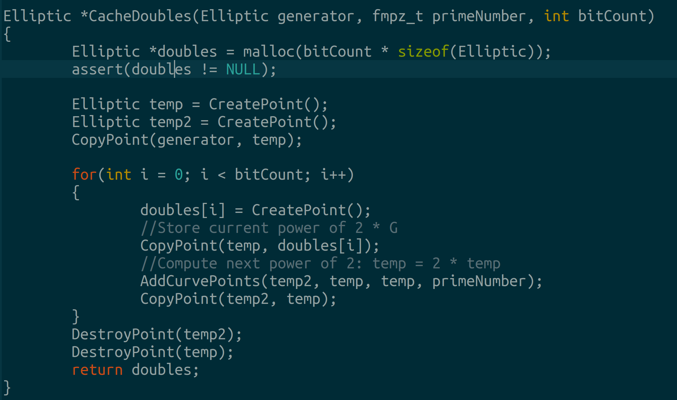
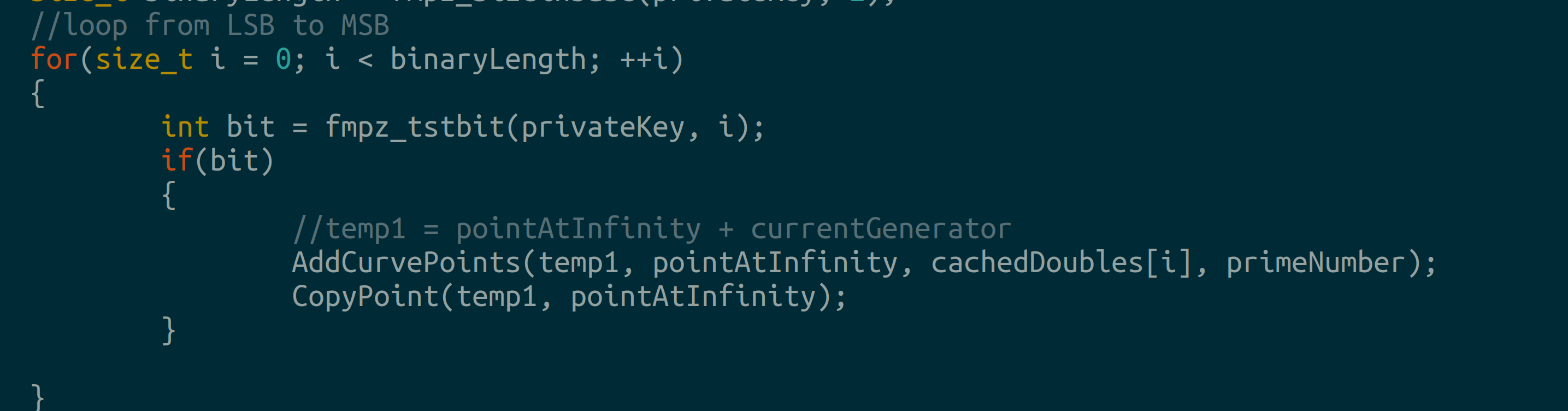
Utilising this LUT rids us of doubling at each step. Our new LSB scalar multiplication loop resembles this:
Remember, libsecp256k1 took ~2.9 seconds for 100,000 keys. Simple caching places us at ~2.7 seconds! Already winning lol.
At this point, the number of additions is linearly proportional to the number of one’s in the binary representation of our scalar. For instance, for a 130 bit private key, we would perform 130 additions at most.
2.3 Finding Integer Primitive Roots
Our previous section got rid of point doublings. In reality, we in fact want to have more doublings than additions. This section demonstrates a better approach to bruteforcing lots of keys.
In group theory, a generator or a primitive element is an element of a finite field that can produce all other elements in the field through repeated multiplication (Kibicho, 2025)3.
For example, in an integer finite field modulo 5, the number 2 is a generator, So, the powers of 2 uniquely produce all elements in the field: 2¹ = 2, 2² = 4, 2³ = 3, 2⁴ = 1.
Below is a programmer’s introduction to generators:

We can find a primitive root modulo the curve’s generator order (not the entire curve’s order) and use this to generate unique points.
The order of the secp256k1 generator point is given in the offical SEC whitepaper (Certicom, 2010)4:
n = 0xFFFFFFFFFFFFFFFFFFFFFFFFFFFFFFFEBAAEDCE6AF48A03BBFD25E8CD0364141n is prime so finding a primitive root, g, is pretty easy:
Find the prime factorization of n-1.
For each distinct prime factor, q, check to ensure that the generator raised to (n-1) divided by q is congruent to 1:

Test for generators If we find a primitive root then we can uniquely represent all points generated by our starting point as:


To double effectively, we need primitive roots either as mersenne primes (OEIS, 2024)5 or fermat primes (Weisstein, 2025)6.

This ensures operations are doubles, with a single addition at the end.
*In a finite field, addition and subtraction are the same thing
For example:
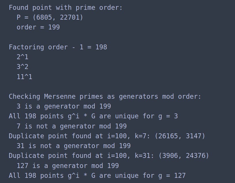
Take the curve y2 = x3 + 7 modulo the prime 38851.
Take the generator P = (6805, 22701) of order 199.
Factor (199-1) = 198 into 21 • 32 • 111.
For a list of primes, perform the power test.
We get for point P that 3 and 127 are primitive roots. Other primes do not generate unique points

Python proof of concept
2.4 Reducing Overall Additions
Sweet! We found mersenne-style primitive roots modulo our generator’s order in the previous section. Now, we use this to reduce the overalll additions in our library.
Here’s our thesis: we need only p doubles and 1 addition* to find successive random points when our primitive root is either a mersenne or fermat prime.
*In a finite field, addition and subtraction are the same operation

We derive the formula below:

In C, our new scalar multiplication algorithm resembles this:
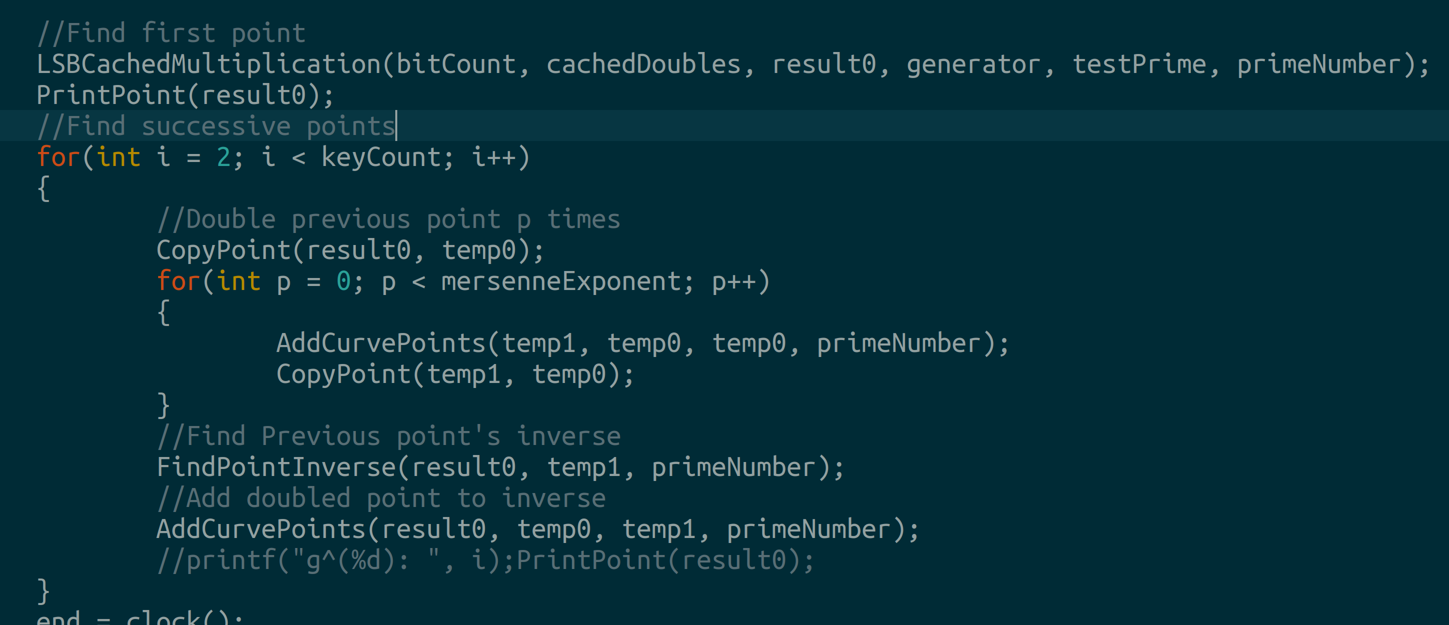
Lo and behold. Using the mersenne prime, 2^7 our total time for 100,000 keys is 0.2651 seconds (about 381430 keys/sec):
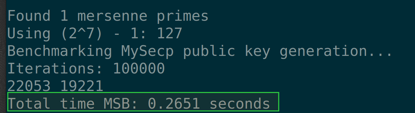
Our estimator script places us at 12.26 million years lol! We shaved off 310 million years lol.

This guides us to the conclusion: we need to focus on reducing the search space.
Note that, if we start from a point with a know scalar, like Q = MP, then we can find a closed form expression for each step:

This says, if I start from the public key M and land on a point whose scalar I know, then I can solve for M.

If M values are within a known range then this gives a 'lift map' of sorts.
It also lets us avoid the recurrence entirely. We can double to get to anywhere

3.1 Custom Collision Finding Algorithm
In Chapter 6, we implemented the Pollard-Rho paper (Pollard, 1978)7 from scratch and wrote an elliptic curve discrete log solver.
Both algorithms were disappointing because:
Pollard Rho for elliptic curves is extremely slow.
Lots of implementation gotchas. No honestly. Each step in the elliptic algo is more of “hand-wavy idk why it works. it just does”.
Pollard Kangaroo/Lambda fails quite often on elliptic curves. You’re not assured you’ll solve the discrete log problem with this algo.
Afterwards, we implemented Pohlig-Hellman here and observed: Pohlig-Hellman works best when p-1 factors pleasantly.
This section combines the good parts of Pollard Rho, Pollard Kangaroo and Pohlig-Hellman for a custom bitcoin-puzzle solver.
Here’s our thesis: we can find elliptic curve point collisions by raising our primitive roots to different powers.
We can find the value of x by solving:

So our version of Pollard-Kangaroo will solve the elliptic curve DLP and this is the equation to solve!
Amazing! We’re at 12.5 million years. Now we’re done with math optimizations. In the next chapter we shall add assembly and CUDA.
Here are some free GPU credits from Runpod.


