IBM Patented Euler's 200 year old Math Technique

Quick Intro

LeetArxiv is a successor to Papers With Code after the latter shutdown.

Quick Summary

IBM owns the patent to the use of derivatives to find the convergents of a generalized continued fraction.

Here’s the bizarre thing: all they did was implement a number theory technique by Gauss, Euler and Ramanujan in PyTorch and call backward() on the computation graph.

Now IBM’s patent trolls can charge rent on a math technique that’s existed for over 200 years.

As always, code is available on Google Colab and GitHub.

1.0 Paper Introduction

The 2021 paper CoFrNets: Interpretable Neural Architecture Inspired by Continued Fractions (Puri et al., 2021)¹ investigates the use of continued fractions in neural network design.

The paper takes 13 pages to assert: continued fractions (just like mlps) are universal approximators.

The authors reinvent the wheel countless times:

1. They rebrand continued fractions to ‘ladders’.

2. They label basic division ‘The 1/z nonlinearity’.

3. Ultimately, they take the well-defined concept of Generalized Continued Fractions and call them CoFrNets.

Authors rename generalized continued fractions. Taken from page 2 of (Puri et al., 2021)

Honestly, the paper is full of pretentious nonsense like this:

The authors crack jokes while collecting rent on 200 years of math knowledge. Taken from page 2

1.1 Quick Intro to Continued Fraction Expansions

Simple continued fractions are mathematical expressions of the form:

Continued fraction. Taken from John D. Cook

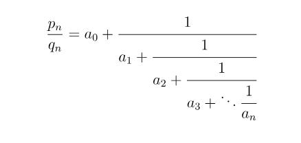
where p_n / q_n is the nth convergent (Cook, 2022)².

Continued fractions have been used by mathematicians to:

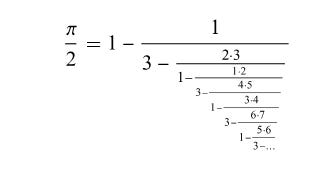
1. Approximate Pi (MJD, 2014)³.

   

   Approximations of Pi taken from WolframAlpha

2. Design gear systems (Brocot, 1861)⁴

   • Achille Brocot, a clockmaker, 1861 used continued fractions to design gears for his watches

3. Even Ramanujan’s math tricks utilised continued fractions (Barrow, 2000)⁵

Continued fractions are well-studied and previous LeetArxiv guides include (Lehmer, 1931)⁶ : The Continued Fraction Factorization Method and Stern-Brocot Fractions as a floating-point alternative.

If your background is in AI, a continued fraction looks exactly like a linear layer but the bias term is replaced with another linear layer.

(Jones, 1980)⁷ defines generalized continued fractions as expressions of the form :

written more economically as :

where a and b can be integers or polynomials.

2.0 Model Architecture

The authors replace the term continued fraction with ‘ladder’ to hide the fact they are reinventing the wheel

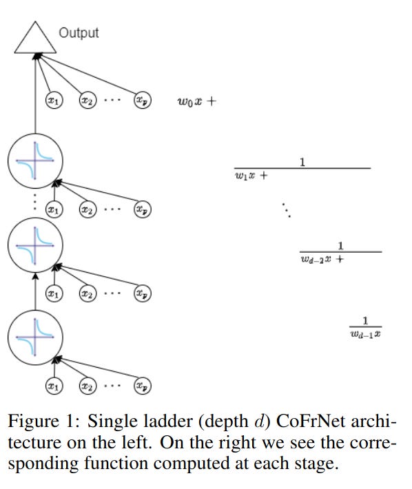
The authors simply implement a continued fraction library in Pytorch and call the backward() function on the resulting computation graph.

That is, they chain linear neural network layers and use the reciprocal (not RELU ) as the primary non-linearity.

Then they replace the bias term of the current linear layer with another linear layer. This is a generalized continued fraction.

In Pytorch, their architecture resembles this:

import torch
import torch.nn as nn
import torch.optim as optim
from sklearn.datasets import make_classification
from sklearn.model_selection import train_test_split
from sklearn.preprocessing import StandardScaler
import numpy as np

class CoFrNet(nn.Module): 
    def __init__(self, input_dim, num_ladders=10, depth=6, num_classes=3, epsilon=0.1):
        super(CoFrNet, self).__init__()
        self.depth = depth
        self.epsilon = epsilon
        self.num_classes = num_classes

        #Linear layers for each step in each ladder
        self.weights = nn.ParameterList([
            nn.Parameter(torch.randn(num_ladders, input_dim)) for _ in range(depth + 1)
        ])

        #Output weights for each class
        self.output_weights = nn.Parameter(torch.randn(num_ladders, num_classes))

    def safe_reciprocal(self, x):
        return torch.sign(x) * 1.0 / torch.clamp(torch.abs(x), min=self.epsilon)

    def forward(self, x):
        batch_size = x.shape[0]
        num_ladders = self.weights[0].shape[0]

        # Compute continued fractions for all ladders
        current = torch.einsum(’nd,bd->bn’, self.weights[self.depth], x)

        # Build continued fractions from bottom to top
        for k in range(self.depth - 1, -1, -1):
            a_k = torch.einsum(’nd,bd->bn’, self.weights[k], x)
            current = a_k + self.safe_reciprocal(current)

        # Linear combination for each class
        output = torch.einsum(’bn,nc->bc’, current, self.output_weights)
        return output

def test_on_waveform():
    # Load Waveform-like dataset
    X, y = make_classification(
        n_samples=5000, n_features=40, n_classes=3, n_informative=10,
        random_state=42
    )

    # Split data
    X_train, X_test, y_train, y_test = train_test_split(X, y, test_size=0.3, random_state=42)

    # Standardize
    scaler = StandardScaler()
    X_train = scaler.fit_transform(X_train)
    X_test = scaler.transform(X_test)

    # Convert to torch tensors
    X_train = torch.FloatTensor(X_train)
    X_test = torch.FloatTensor(X_test)
    y_train = torch.LongTensor(y_train)
    y_test = torch.LongTensor(y_test)

    # Model
    input_dim = 40
    num_classes = 3
    model = CoFrNet(input_dim, num_ladders=20, depth=6, num_classes=num_classes)

    # Training
    criterion = nn.CrossEntropyLoss()
    optimizer = optim.Adam(model.parameters(), lr=0.001)

    epochs = 100
    batch_size = 64

    for epoch in range(epochs):
        model.train()
        permutation = torch.randperm(X_train.size()[0])

        for i in range(0, X_train.size()[0], batch_size):
            indices = permutation[i:i+batch_size]
            batch_x, batch_y = X_train[indices], y_train[indices]

            optimizer.zero_grad()
            outputs = model(batch_x)
            loss = criterion(outputs, batch_y)
            loss.backward()
            optimizer.step()

        # Validation
        if epoch % 10 == 0:
            model.eval()
            with torch.no_grad():
                train_outputs = model(X_train)
                train_preds = torch.argmax(train_outputs, dim=1)
                train_acc = (train_preds == y_train).float().mean()

                test_outputs = model(X_test)
                test_preds = torch.argmax(test_outputs, dim=1)
                test_acc = (test_preds == y_test).float().mean()

            print(f’Epoch {epoch:3d} | Loss: {loss.item():.4f} | Train Acc: {train_acc:.4f} | Test Acc: {test_acc:.4f}’)

    print(f”\nFinal Test Accuracy: {test_acc:.4f}”)
    return test_acc.item()

if __name__ == “__main__”:
    accuracy = test_on_waveform()
    print(f”CoFrNet achieved {accuracy:.1%} accuracy on Waveform dataset”)

3.0 Results

Testing on a non-linear waveform dataset, we observe these results:

CoFrNet learns a non-linear dataset

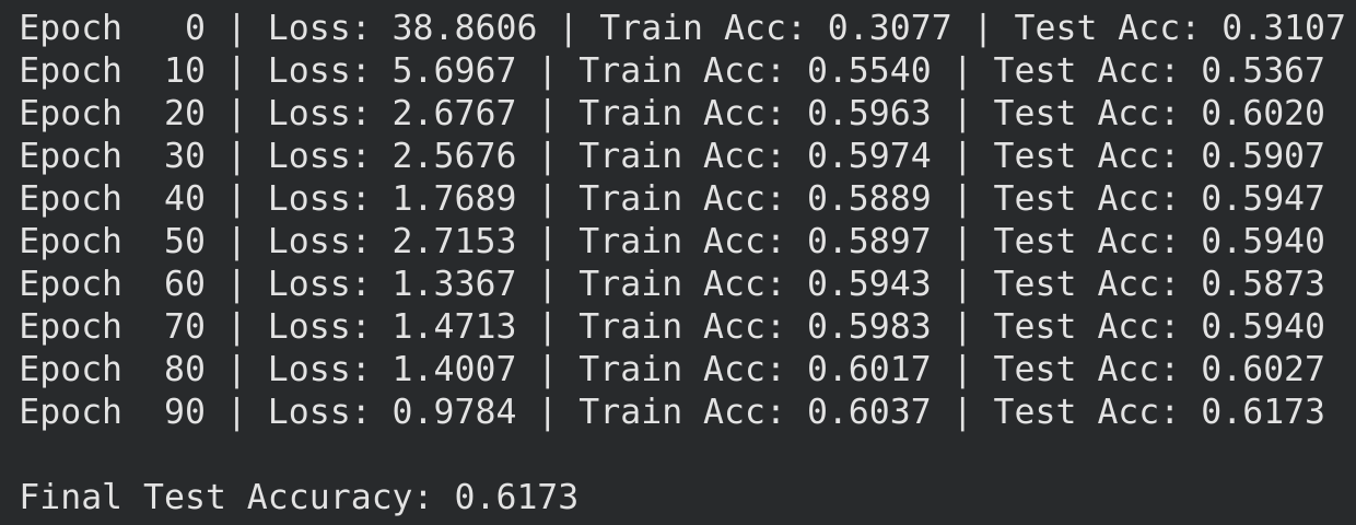
An accuracy of 61%.

Nowhere near SOTA and that’s expected.

Continued fractions are well-studied and any number theorist would tell you the gradients vanish ie there are limits to the differentiability of the power series.

The authors use power series of continued fractions to interpret their moderate success. Taken from page 6 of (Puri et al., 2021)

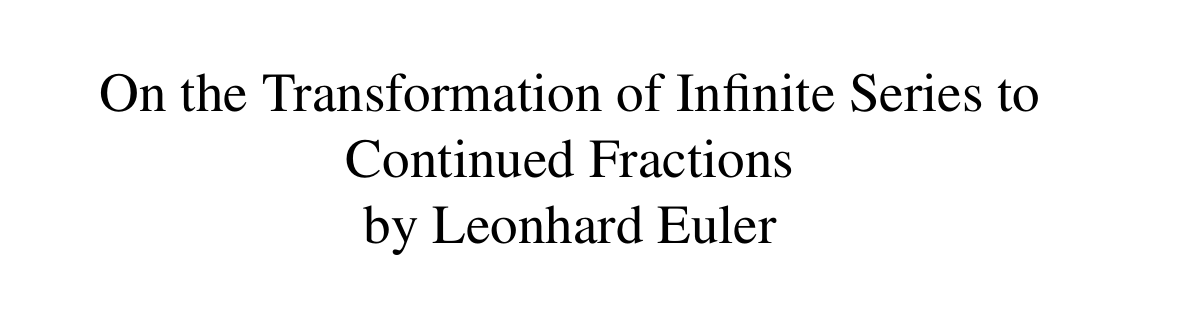
Even Euler’s original work (Euler, 1785)⁸ allude to this fact: it is an infinite series so optimization by differentiation has its limits.

Pytorch’s autodiff engine replaces the differentiabl series with a differentiable computational graph.

The authors simply implemented a continued fraction library in Pytorch and as expected, saw the gradients could be optimized.

4.0 The Patent

Patent application for Continued Fractions. Taken from Justia Patents

As the reviewers note, the idea seems novel but the technique is nowhere near SOTA and the truth is, continued fractions have existed for a while. They simply replace the linear layers of a neural network with generalized continued fractions.

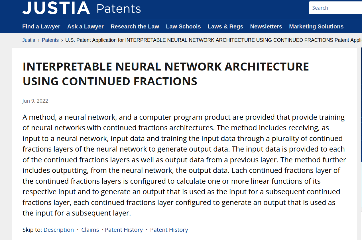
Here’s the bizarre outcome: the authors filed for a patent on their ‘buzzword-laden’ paper in 2022.

The patent has been published on Google Patents.

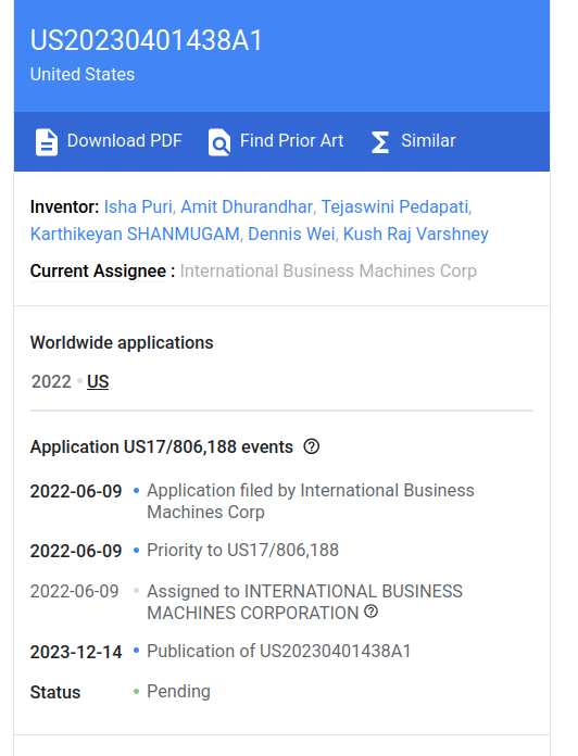
Their patent was published and its status marked as pending.

Here’s the thing:

1. Continued fractions have existed longer than IBM.

2. Differentiablity of continued fractions is well-known.

3. The authors did not do anything different from Euler’s 1785 work.

   • Generalized continued fractions can take anything as inputs. It can be integers, or the CIFAR-10 dataset. That’s what the ‘generalized’ means.

Now, If IBM feels litigious they can sue Sage, Mathematica, Wolfram or even you for coding a 249 year old math technique.

4.1 Who is affected by IBM’s Patent?

1. Mechanical engineers, Robotics and Industrialists

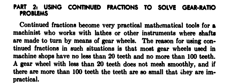
   • Continued fractions are used to find the best number of teeth for interlocking gears (Moore, 1964)⁹. If you happen to use the derivative to optimize your fraction selection then you’re affected

   

   Taken from page 30 of An Introduction to Continued Fractions (Moore, 1964)

2. Pure Mathematicians and Math Educators

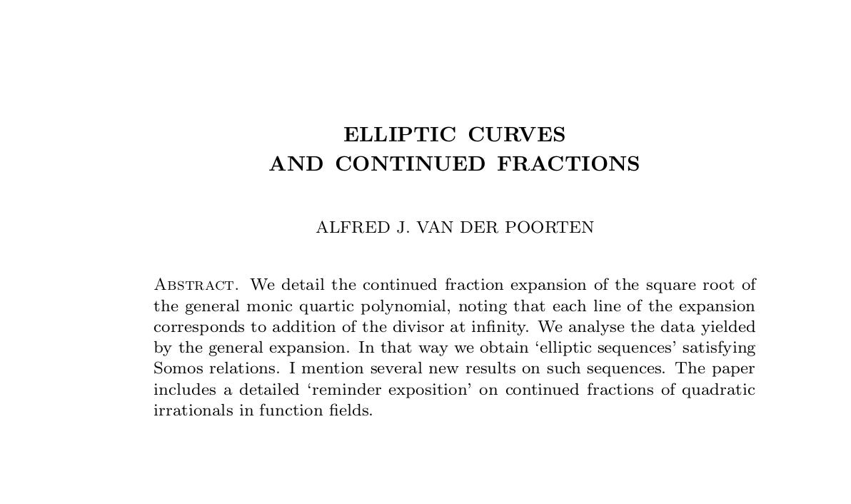
   I’m a Math PhD and I learnt about the patent while investigating Continued Fractions and their relation to elliptic curves (van der Poorten, 2004)¹⁰.

   I was trying to model an elliptic divisibilty sequence in Python (using Pytorch) and that’s how I learnt of IBM’s patent.

   

   Abstract for the 2004 paper Elliptic Curves and Continued Fractions (van der Poorten, 2004)

3. Numerical Analysts and Computation Scientists/Sage and Maple Programmers

   Numerical analysis is the use of computer algorithms to approximate solutions to math and physics problems (Shi, 2024)¹¹.

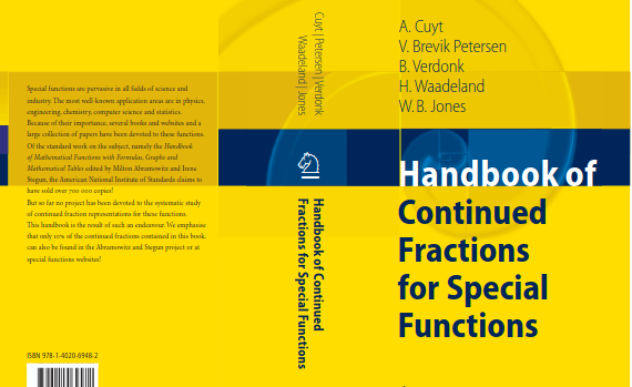
   Continued fractions are used in error analysis when evaluating integrals and entire books describe these algorithms (Cuyt et al., 2008)¹².

   

References

1. Puri, I., Dhurandhar, A., Pedapati, T., Shanmugam, K., Wei, D., & Varshney, K. R. (2021). CoFrNets: Interpretable neural architecture inspired by continued fractions. In A. Beygelzimer, Y. Dauphin, P. Liang, & J. Wortman Vaughan (Eds.), Advances in neural information processing systems. https://openreview.net/forum?id=kGXlIEQgvC

2. Cook, J. (2022). Continued fractions as matrix products. Blog Post.

3. MJD. (2014). How to find continued fraction of pi. Mathematics Stack Exchange. https://math.stackexchange.com/q/716976

4. Brocot, A. (1861). Calcul des rouages par approximation, Nouvelle méthode. Revue chronomeétrique, 3. 186-94.

5. Barrow, J. (2000). Chaos in Numberland: The secret life of continued fractions. Link.

6. Jones, William B., and W. J. Thron (1980). Continued Fractions: Analytic Theory and Applications. Cambridge University Press.

7. Lehmer, D. H., & Powers, R. E. (1931). On factoring large numbers. Bulletin of the American Mathematical Society, 37(10), 770–776.

8. Euler, L. (1785). De transformatione serierum in fractiones continuas, ubi simul haec theoria non mediocriter amplificatur (D. W. File, Trans., 2004). Department of Mathematics, The Ohio State University. (Original work published 1785)

9. Moore, C. (1964). An Introduction to Continued Fractions. National Council of Teachers of Mathematics. Link.

10. van der Poorten, A. J. (2004). Elliptic curves and continued fractions [Preprint]. arXiv. https://arxiv.org/abs/math/0403225

11. Shi, A., (2024). Numerical Analysis (Math 128a). UC Berkeley. Link.

12. Cuyt, A., Petersen, V. B., Verdonk, B., Waadeland, H., & Jones, W. B. (2008). Handbook of continued fractions for special functions. Springer.