Bleichenbacher Attacks on Hidden Number Problems

Quick Summary

We code in the C programming language a Fourier Analysis approach to solving hidden number problems.

Abstract for the 2014 paper, GLV/GLS Decomposition, Power Analysis, and Attacks on ECDSA Signatures with Single-Bit Nonce Bias (Aranha et al., 2014) that demonstrates the Bleichenbacher solution to HNPs

This is part of our series on Practical Hidden Number Problems for Programmers:

*These links are paywalled. (It’s how I’ll afford grad school lol)

Part 1: Quantum Computing and Intro to Hidden Number Problems

Part 2: Increasing Lattice Volume for Improved HNP Attacks

Part 3: Hidden Number Problems with Multiple Noise Holes

Part 4: Hidden Number Problems with Chosen Multipliers

Part 5: Hidden Number Problems with Chosen Errors

Part 6 : Solving Hidden Number Problems Without Lattices

Part 7 (we are here) : Fourier Analysis Attacks on HNPs

As usual, code is available on GitHub.

1.0 Introduction

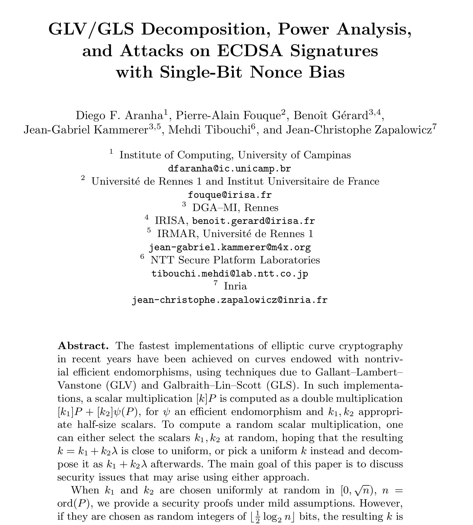
The 2014 paper GLV/GLS Decomposition, Power Analysis, and Attacks on ECDSA Signatures with Single-Bit Nonce Bias (Aranha et al., 2014)¹ demonstrates Bleichenbacher’s approach to solving hidden number problems (HNPs) using fourier analysis.

Lattices need at least 2 leaked bits. Taken from “Our Contributions’ section of (Aranha et al., 2014)

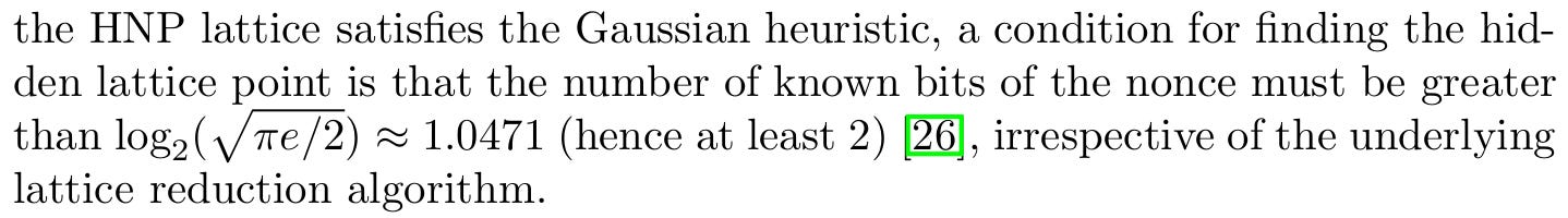
The lattice approaches explored in Part 1 to Part 5 can’t solve single-bit leaks because the corresponding HNP solultion will not be the closest vector even under the Gaussian Heuristic (Aranha et al., 2014).

1.1 Bleichenbacher’s Approach

Summary of Bleichenbacher’s Approach. Taken from “Our Contributions’ section of (Aranha et al., 2014)

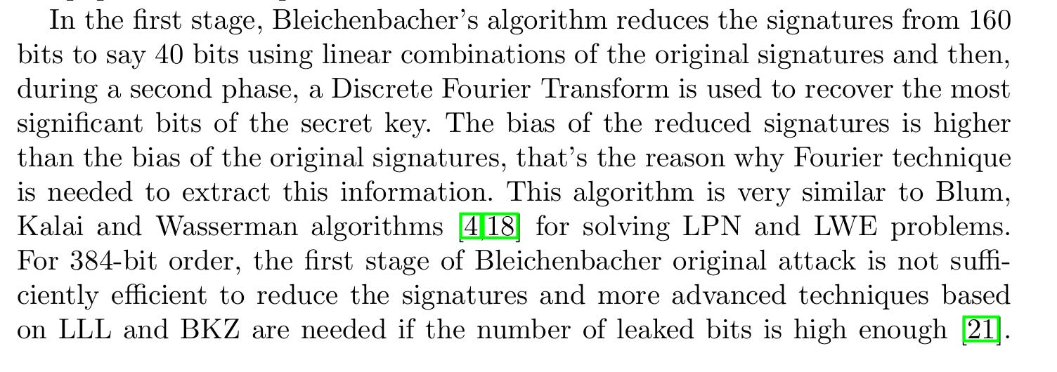
Like every other HNP solution, Bleichenbacher’s approach assumes that the attacker has access to an oracle.

Summary of original approach. Taken from (Mulder et al, 2014)

Bleichenbacher’s approach involves using a bias calculation and an inverse FFT to identify values near the secret key x, thus recovering the MSBs of x (Mulder et al, 2014)² in a HNP of the form:

HNP instance

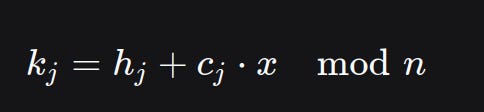
where:

• h_j - known observation (taken from the ECDSA signature)

• c_j - known multiplier (also obtained from the ECDSA signature)

• x - secret key

• k_j - secret noise term (nonce)

2.0 Coding Guide

Bleichenbacher’s attack on HNPs. Taken from Algorithm 2 of (Aranha et al., 2014)

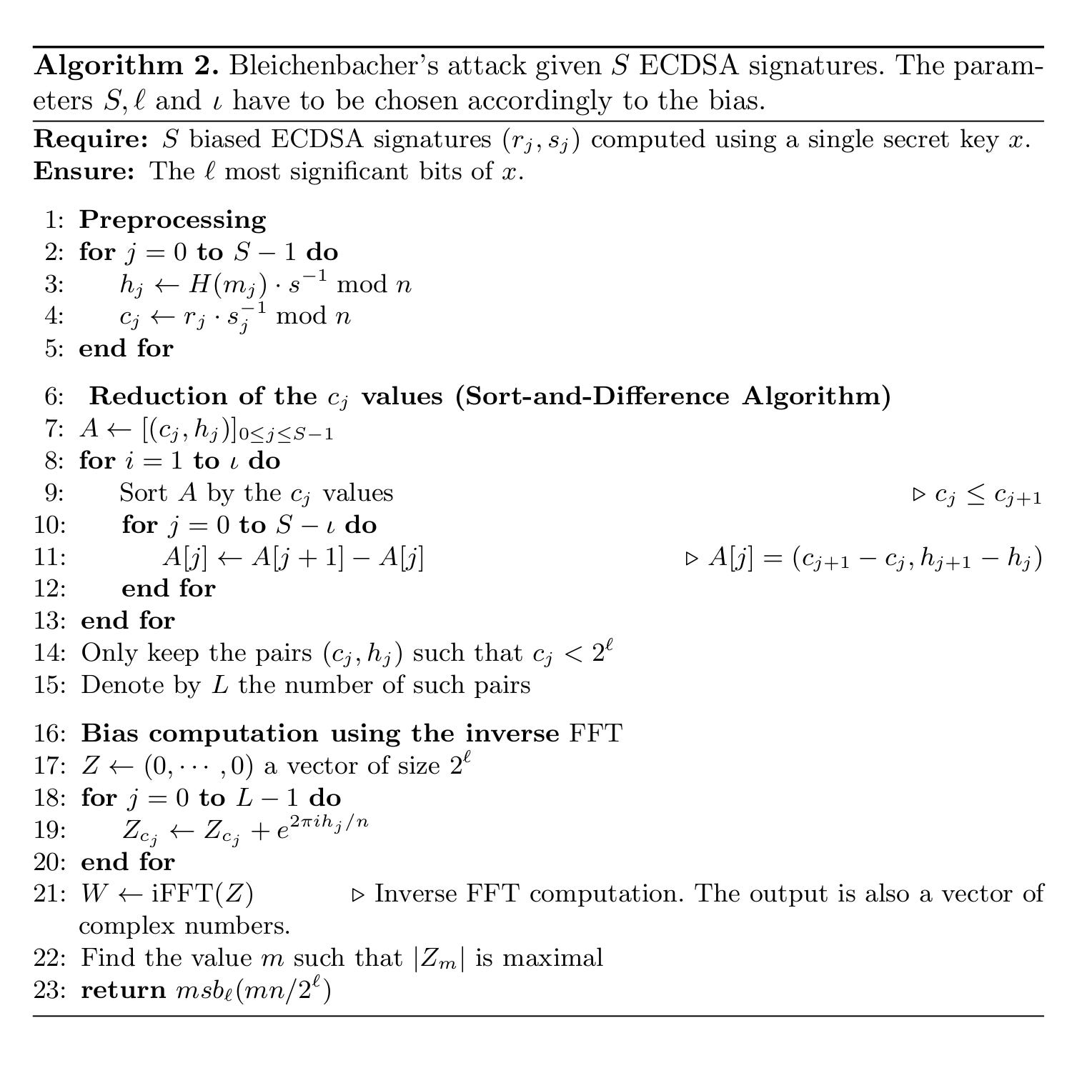
We shall implement Bleichenbacher’s attack on HNPs following algorithm 2 given above.

First, we’ll understand what the bias does. Next, we use the fast fourier transform to speed up the bias calculation.

2.1 Finding Bias Without FFT

The authors introduce bias as a metric for verifying randomness. If we know the number of leaked bits is 1, then the correct secret key should give a bias calculation close to a known target.

The bias is a statistical distinguisher that tells you if your guessed secret key is correct.

Bias definition. Taken from section 2.1 of (Aranha et al., 2014)

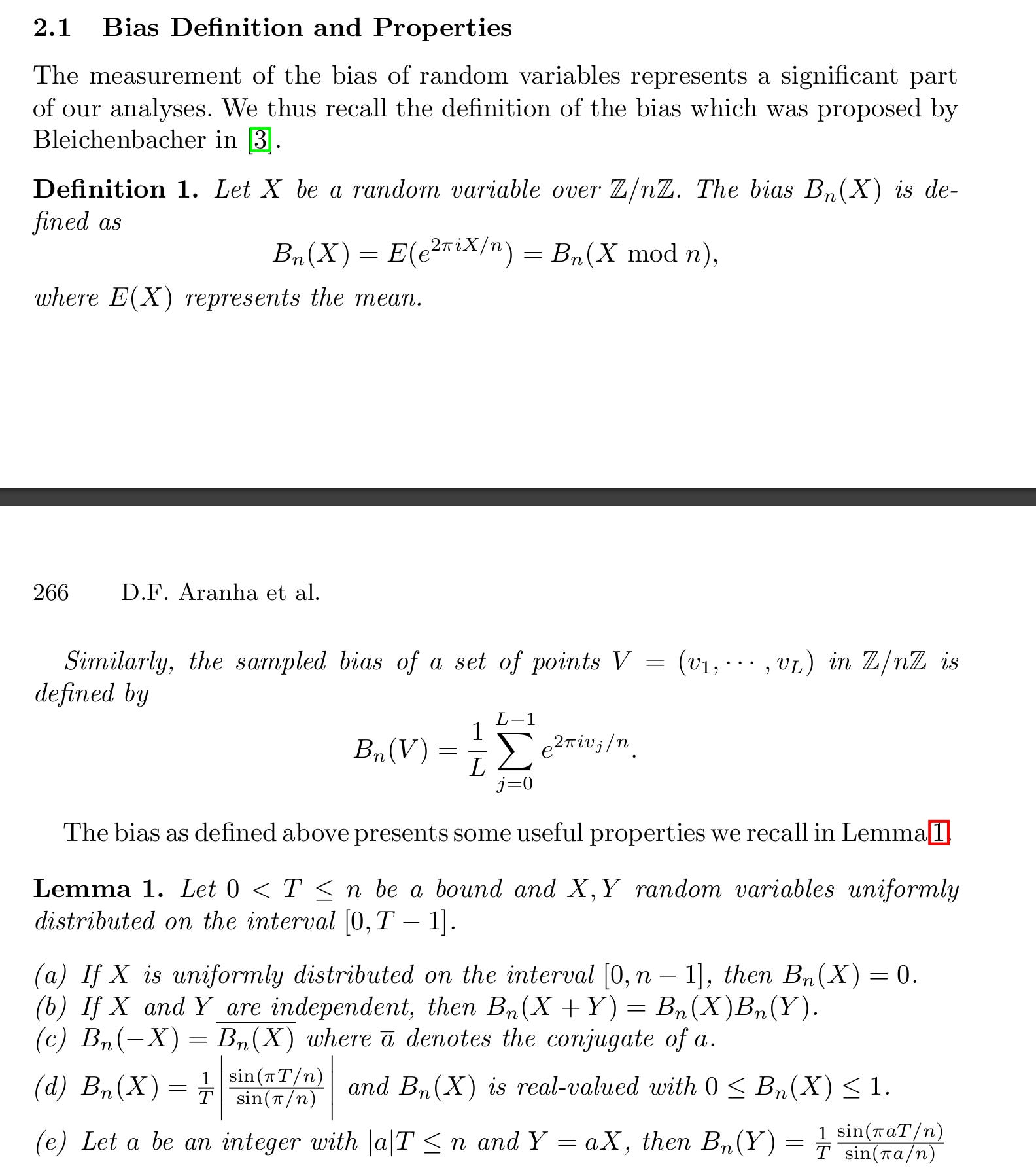
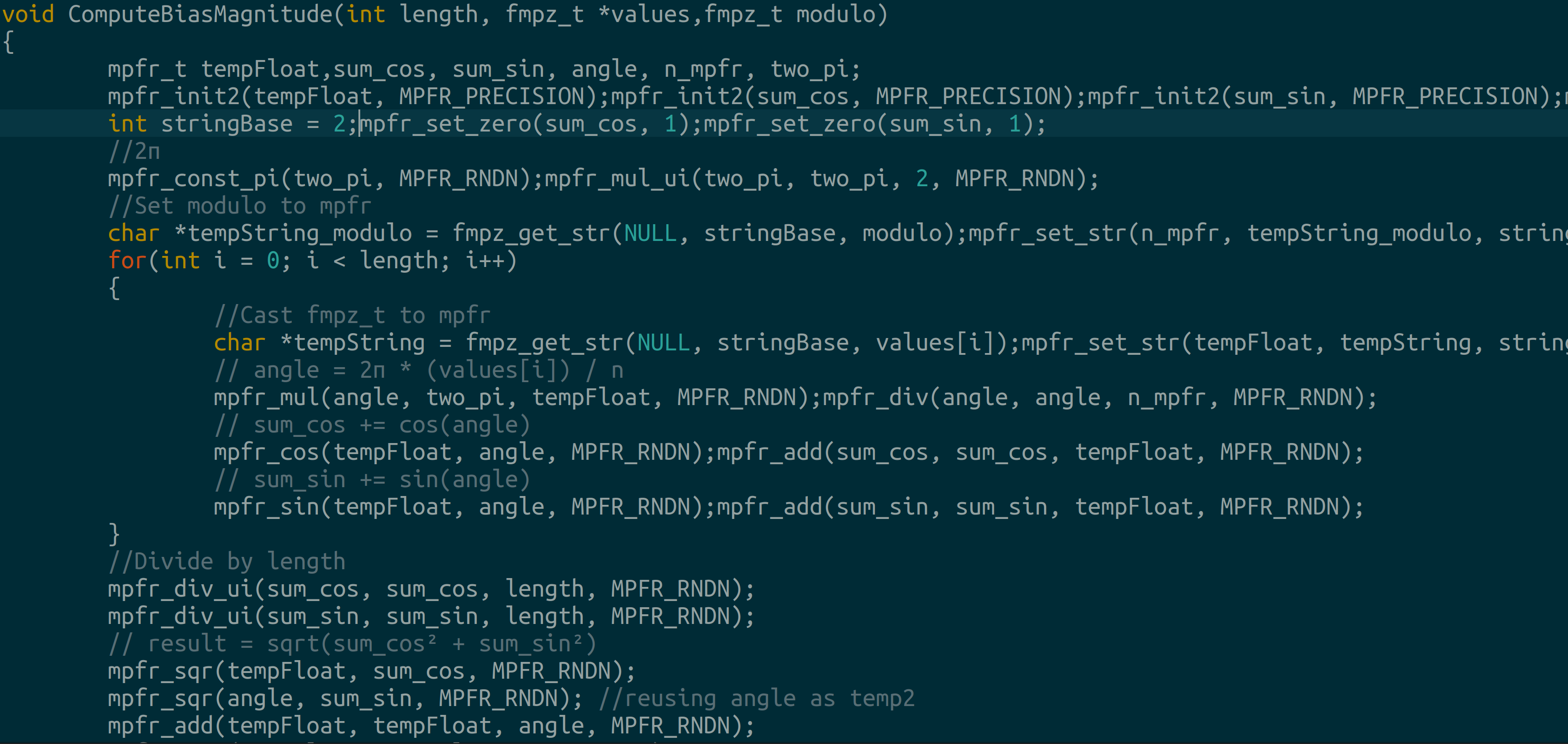
In C, using mpfr, the sampled bias can be calculated by:

Computing bias magnitude

Next, we write a function to test our magnitude computation:

Sample bias magnitude test

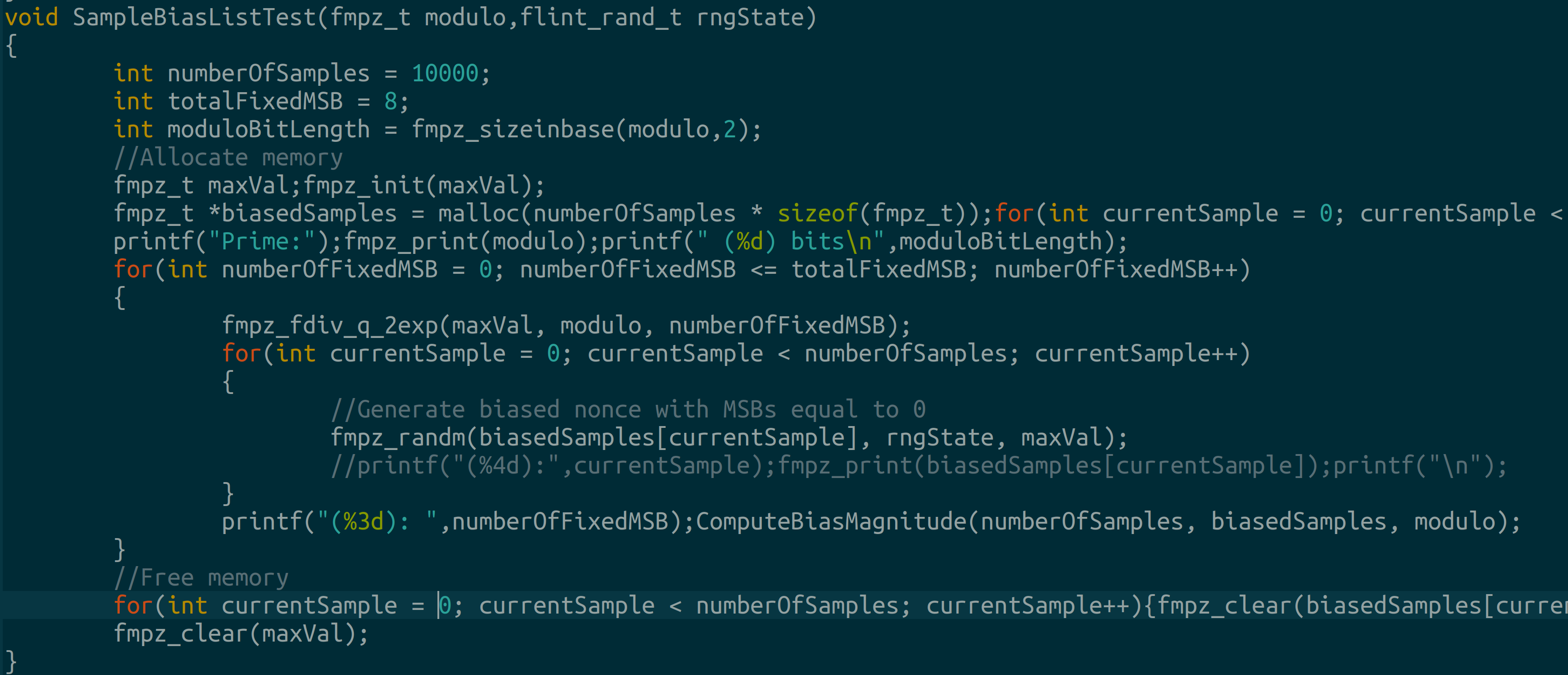
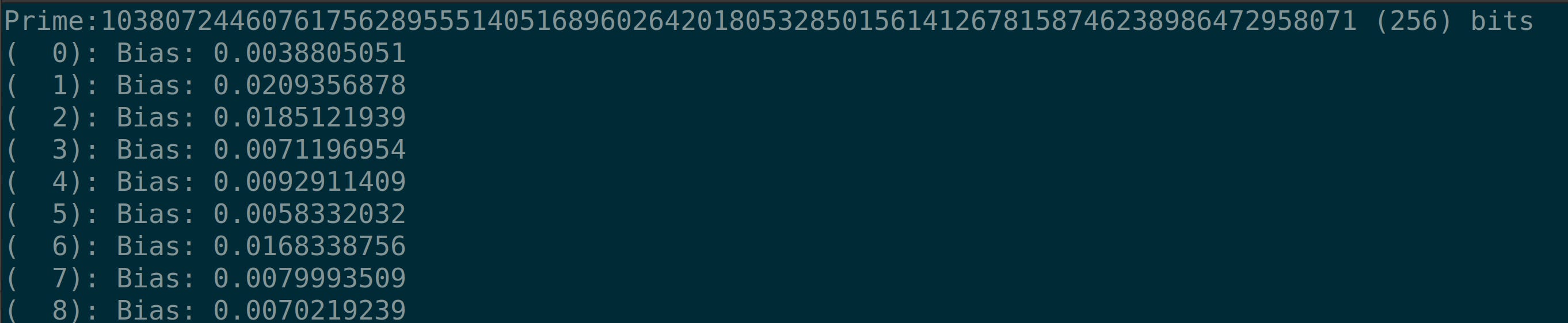
For a 256-bit prime, where the bracketed number represents the number of fixed MSBs, we observe:

Observe how bias magnitude changes with number of fixed MSBs

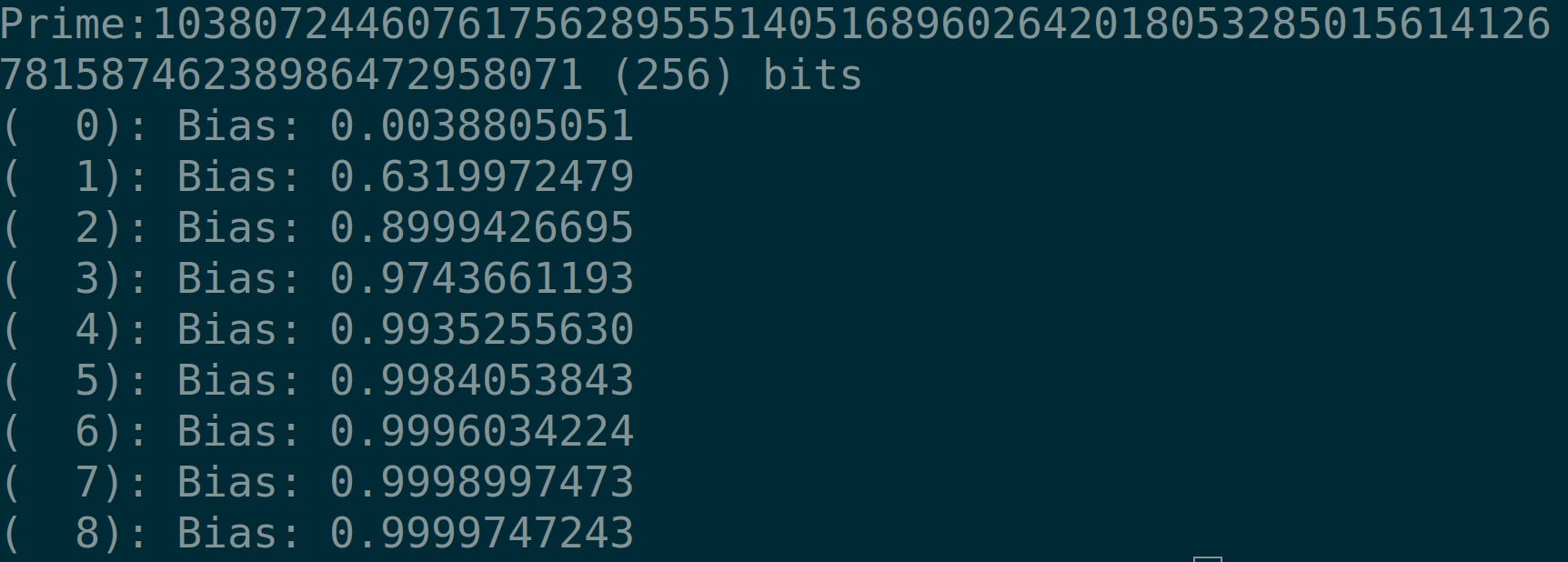
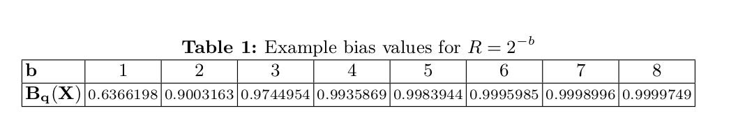
When 0 bits are fixed then the bias should be close to zero. Our results match Table 1:

Example bias values. Taken from (Mulder et al, 2014)

*bias values may be different depending on your RNG

2.1.1 Making Bias Work With LSBs?

An interesting question arises: what if the LSBs, not the MSBs are fixed, will the bias calculation work?

Left shift to sample values with fixed LSBs, not MSBs

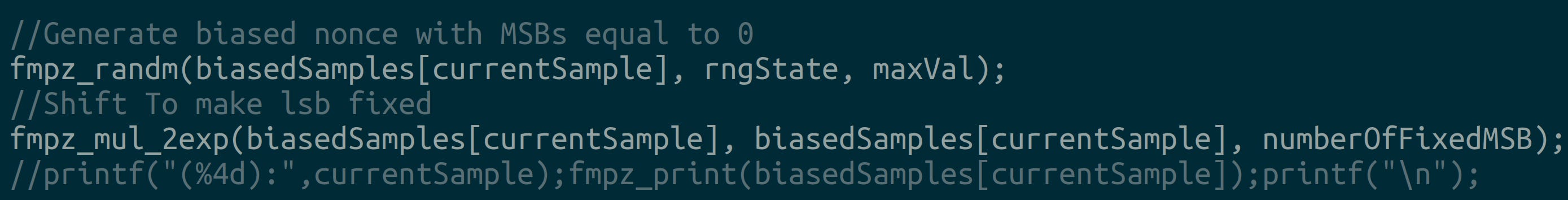
We make the modification above to test it. We observe that the bias function’s results are close to zero for every value:

Naive bias test when LSBs, not MSB are fixed

No, this bias definition is not applicable to fixed LSBs.

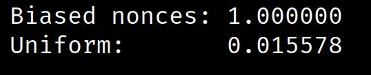
We modify the bias function to work with different fourier coefficients. Here’s the Python code for maximum readability:

We find the optimal frequency corresponding to a fixed MSB case

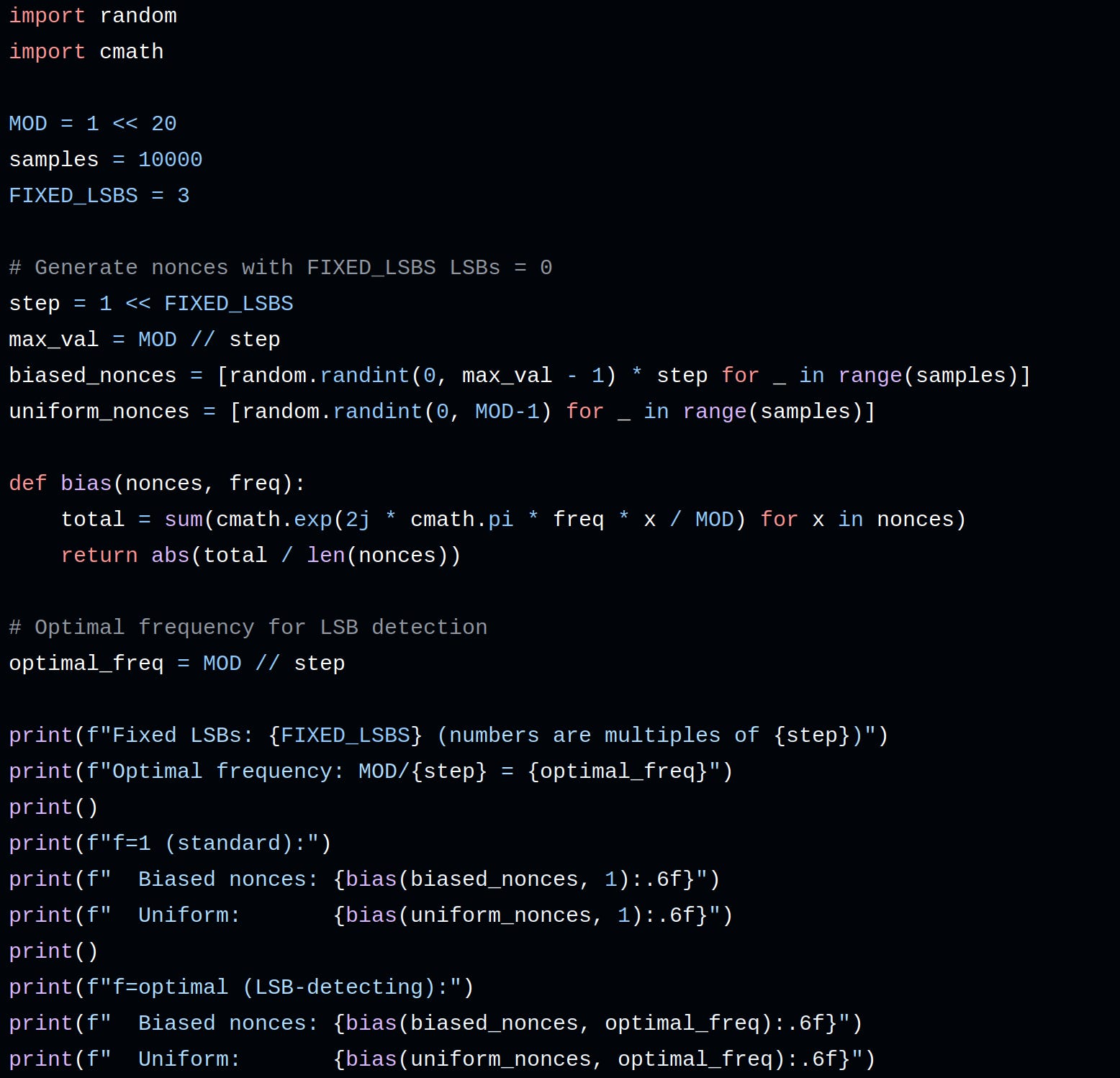
Just like before, the biased LSB nonces are close to 1 while the random nonces are close to zero:

Our modded LSB bias works just like MSB bias

2.2 Connecting HNP to Bias

Relationship between bias and correct solution. Taken from (Mulder et al, 2014)

This is how I understood the connection between HNPs and bias calculations:

1. Say q is small.

2. We can generate a list of possible noise terms where noise = known observation + multiplier * secretKey.

3. Running this generated list through the bias calculator yields a number in the range [0 to 1].

4. The correct secret (or numbers close to the correct secret) show high bias magnitudes.

5. We use the Fast Fourier Transform as a shortcut to evaluate every possible secret key at once.

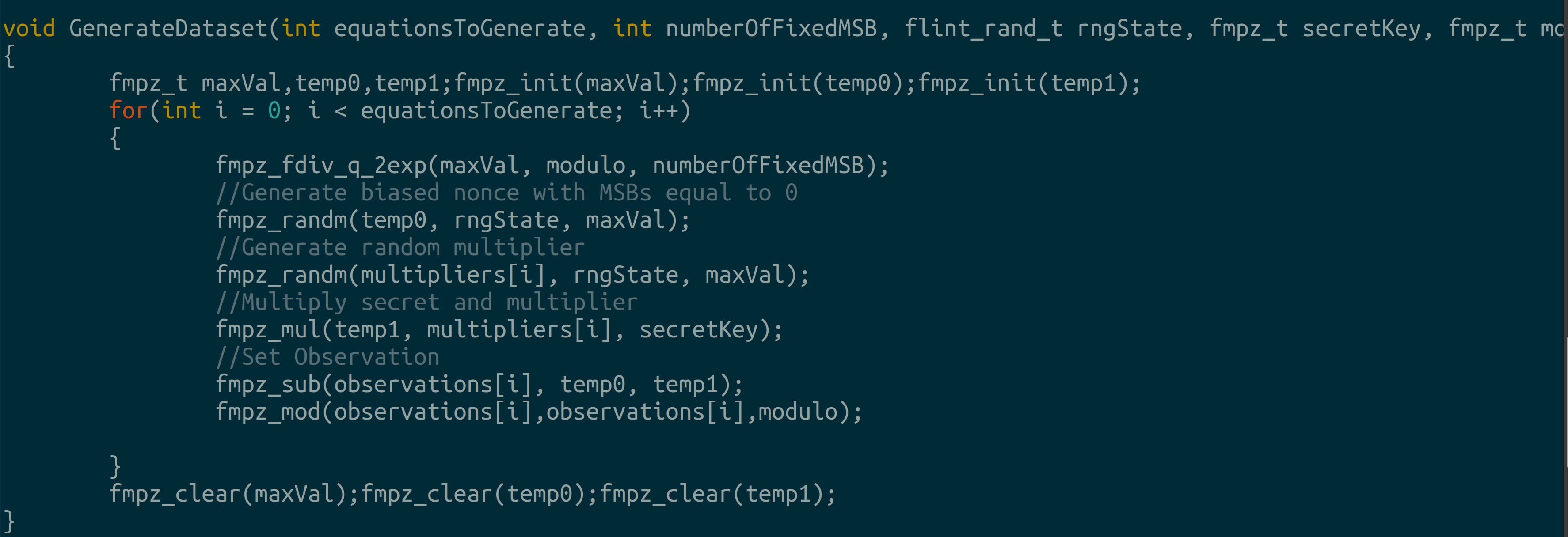
First, we write a function to generate a HNP dataset:

Generate dataset function according to HNP equation

Running this function on a 13 bit prime yields this sample dataset:

Sample dataset

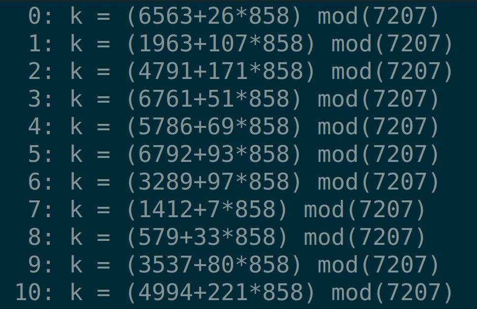
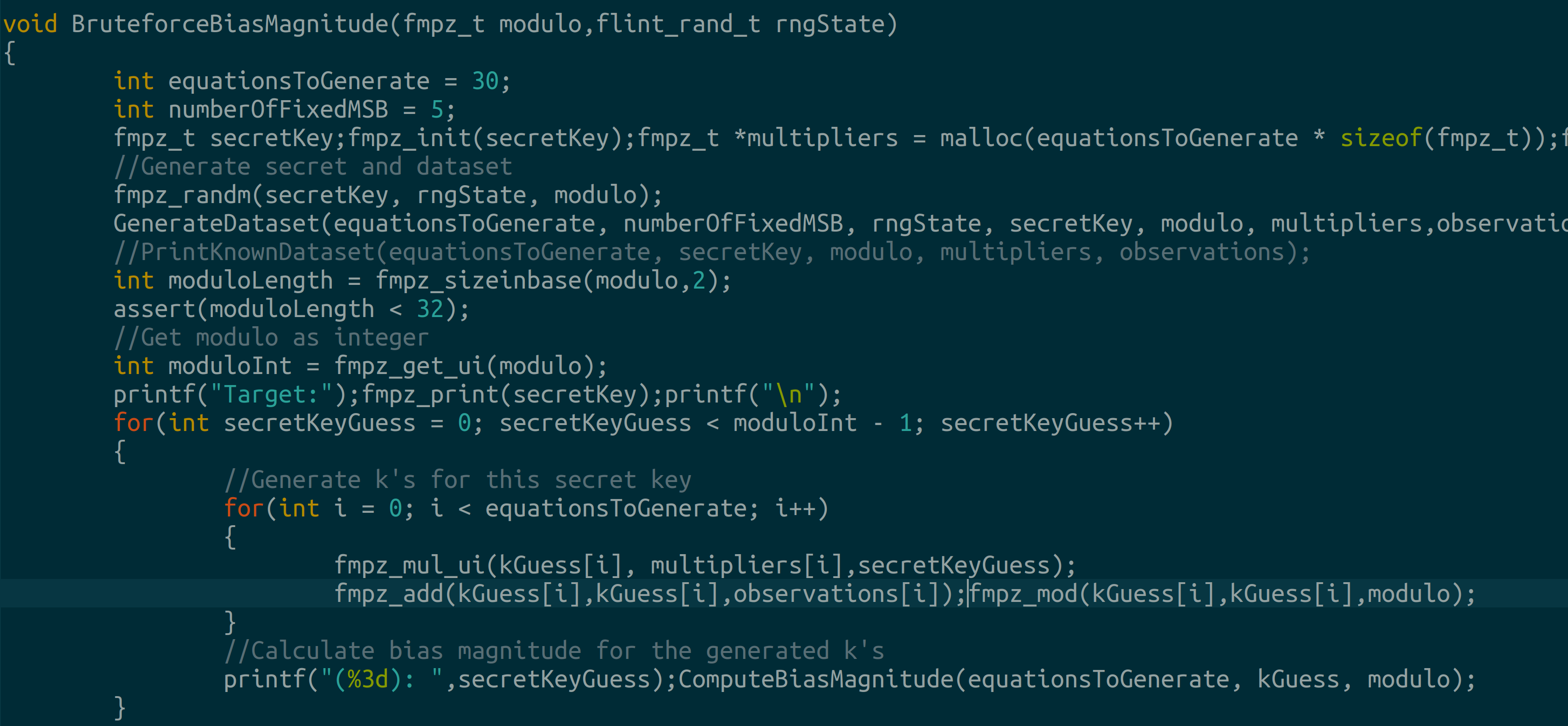
Writing a bruteforcer to permits us grasp Bleichenbacher’s vision: guesses close to the actual secret key demonstrate rather high bias magnitudes.

Function to calculate a bias magnitude for every possible secret key

The unknown secret key is 858 and we observe super large bias magnitudes around 858:

858 and its neighbours demonstrate high bias magnitudes

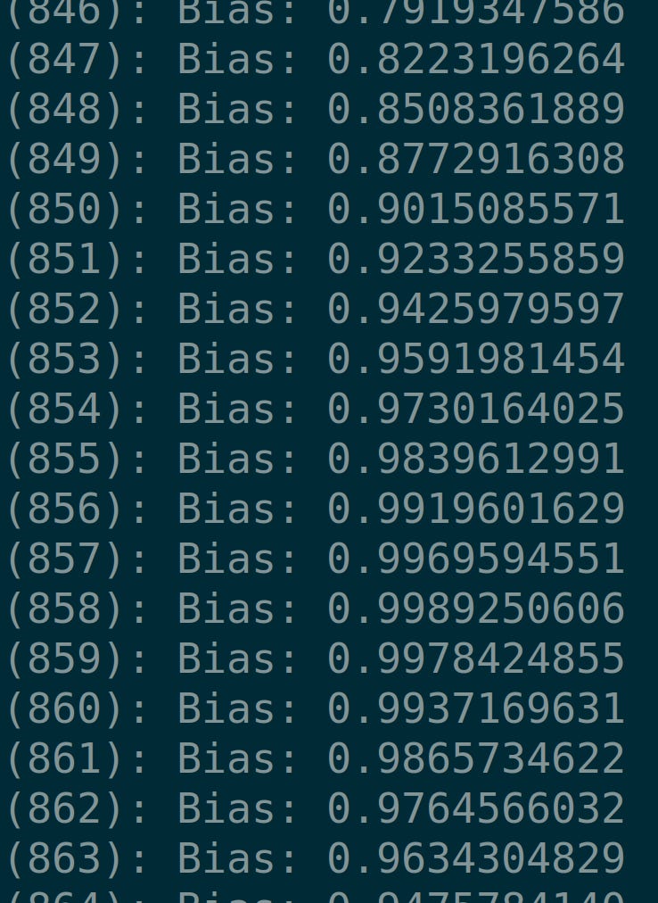
For contrast, the bias magnitudes observed away from 858 are pretty low:

Low bias magnitudes when away from 858

So the bias magnitude tells us when we’re close to the actual secret key.

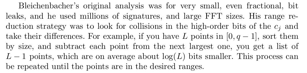
2.2.1 Range Reduction’s Effect on Bias

Sort and Difference. Taken from Algorithm 2 of (Aranha et al., 2014)

The sort and difference reduction algorithm permits us work with small c_j (known multiplier). Each reduction iteration squares the bias. Hence, we can approximated the bias after multiple iterations with:

Approximate bias by repeated squaring. Taken from (Aranha et al., 2014)

That’s the information Table 1 holds:

Table 1. Taken from (Aranha et al., 2014)

Interpret the table’s results as:

Bias decreases with successive sort-and-difference iterations

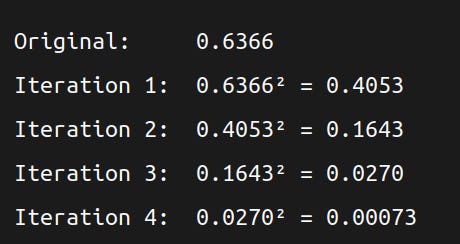
In a nutshell, we can’t run too many sort and difference iterations because the bias would be super small (and appear indistinguishable from the uniform distribution’s bias).

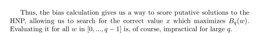
2.3 Using FFT for Fast Bias Calculations

Motivation for FFT approach. Taken from (Mulder et al, 2014)

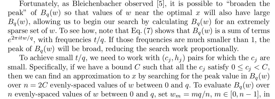
Bruteforce bias search is impractical for large modulos. Instead, we run an n-point FFT on the (observation, multiplier) pair to find the MSB’s we desire.

One may borrow the inplace inverse FFT from (Perry, 2017)³. The FFT is merely a shortcut to finding the bias.

References

1. Aranha, D.F., Fouque, PA., Gérard, B., Kammerer, JG., Tibouchi, M., Zapalowicz, JC. (2014). GLV/GLS Decomposition, Power Analysis, and Attacks on ECDSA Signatures with Single-Bit Nonce Bias. In: Sarkar, P., Iwata, T. (eds) Advances in Cryptology – ASIACRYPT 2014. ASIACRYPT 2014. Lecture Notes in Computer Science, vol 8873. Springer, Berlin, Heidelberg. DOI.

2. De Mulder, E., Hutter, M., Marson, M.E. et al. Using Bleichenbacher’s solution to the hidden number problem to attack nonce leaks in 384-bit ECDSA: extended version. J Cryptogr Eng 4, 33–45 (2014). DOI.

3. Perry, R. (2017). Bleichenbacher Attacks. Website.