Coding Schoof's 1985 Elliptic Curve Point Counting Algorithm in Python

World's First Polynomial Time Algorithm To Count Points On Elliptic Curves

Abstract for Elliptic Curves over Finite Fields and the Computation of Square Roots mod p (Schoof, 1985)

Here’s 20% off scheduling meetings with Cal.com

Here’s 20% off Simplified’s Marketing Agent

1.0 Paper Introduction

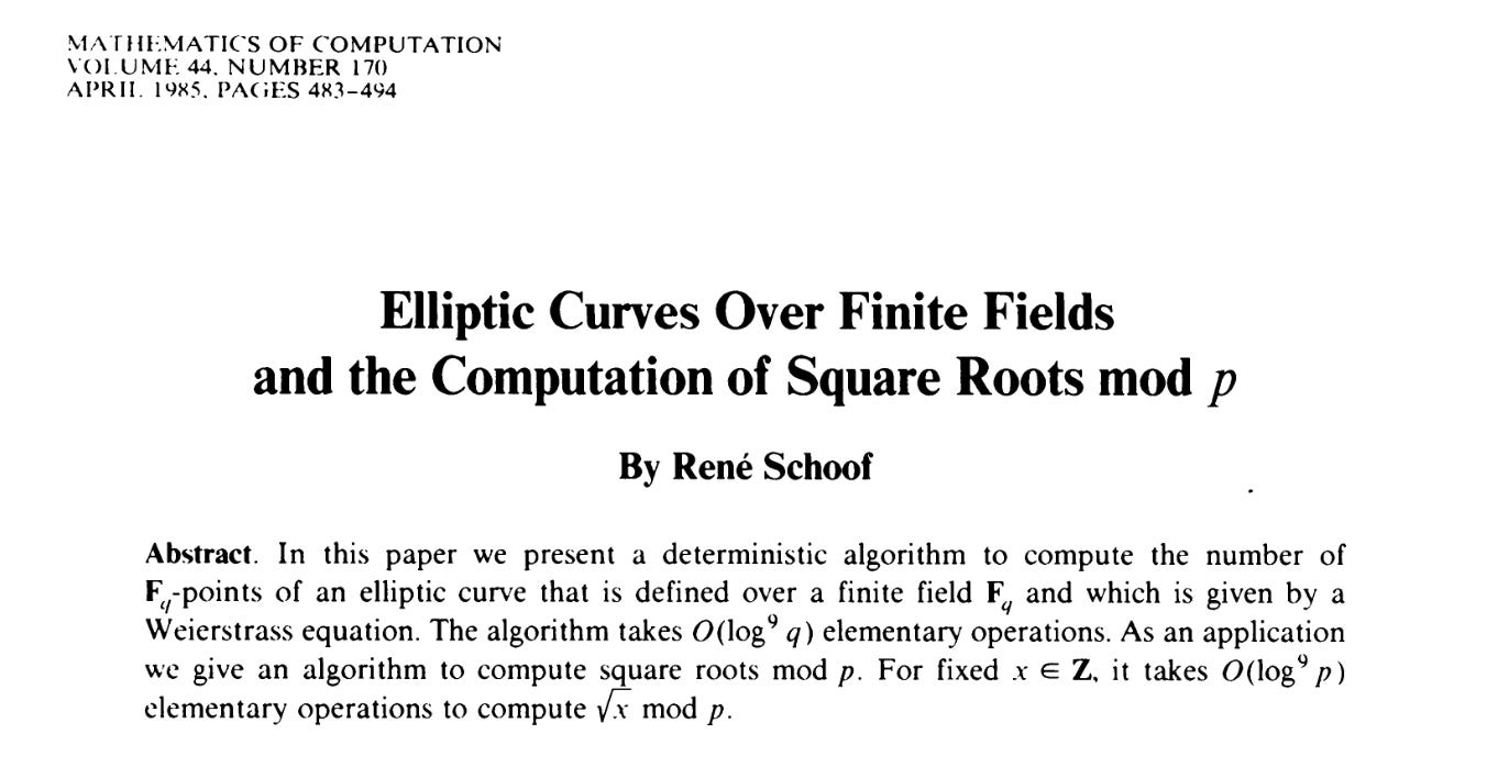
Elliptic Curves over Finite Fields and the Computation of Square Roots mod p (Schoof, 1985)¹ introduced the world’s first polynomial time algorithm to compute the number of points, denoted by #E(F_q), on an elliptic curve (Sutherland, 2025)².

(Schoof, 1985) is canonical because it reduced the complexity of counting points on elliptic curves from exponential to polynomial-time.

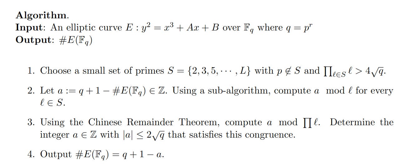
The algorithm is simple: compute the trace of frobenius t modulo many small primes and use the Chinese Remainder Theorem to uniquely determine t (Sutherland, 2025):

Schoof’s algorithm in pseudocode. Taken from page 1 of (Sutherland, 2025)

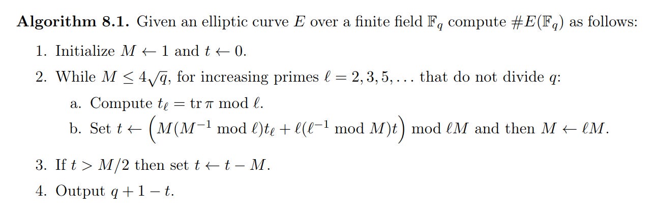
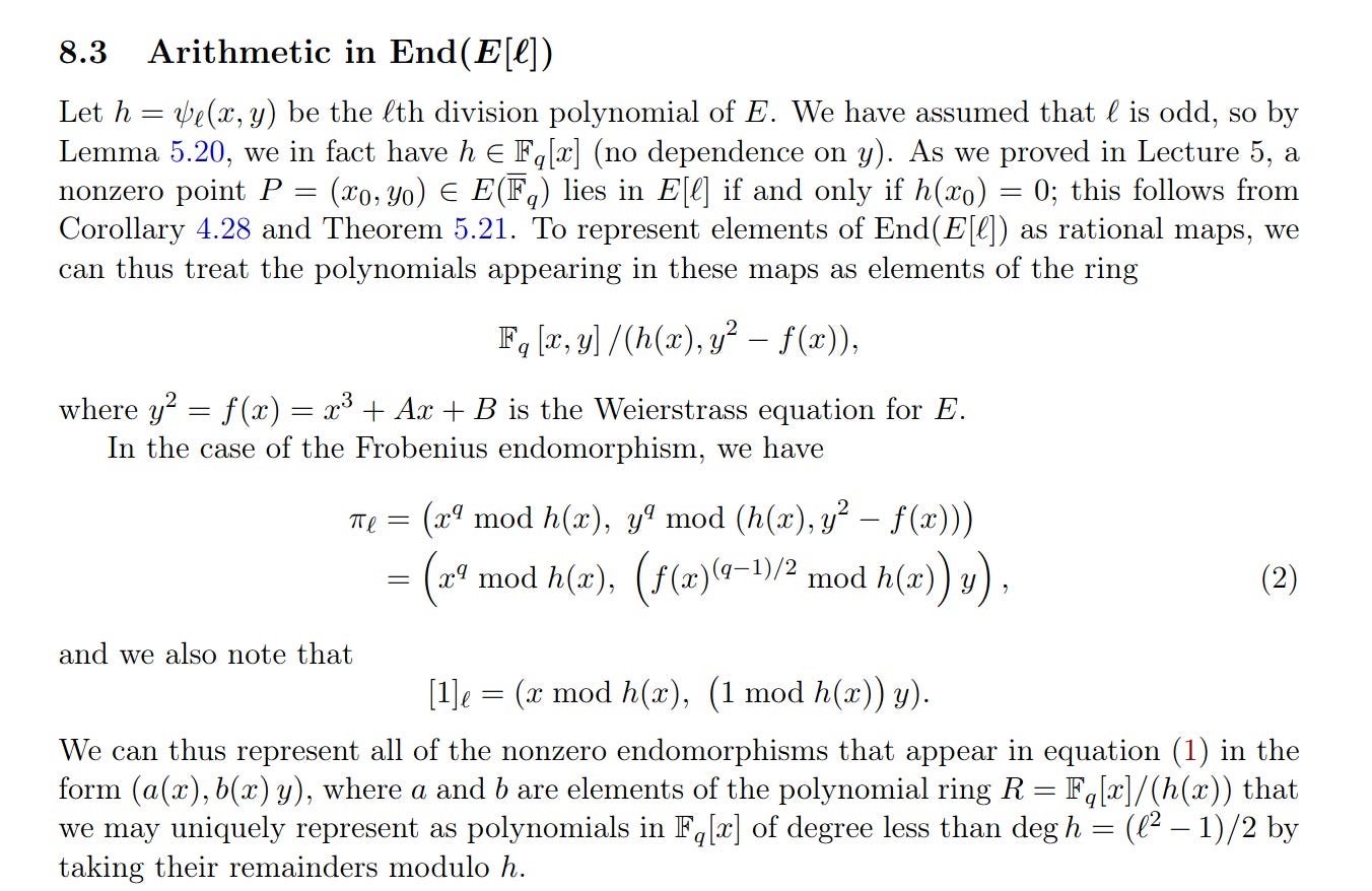
Schoof realized that a curve’s division polynomials identified torsion points modulo small primes. Then he related this to to the frobenius endomorphism. That’s how we got a polynomial-time point counting algo!

Arithmetic in the curve’s endomorphism leads to Schoof’s algorithm. Taken from page 2 of (Sutherland, 2025)

This is part of our series on Practical Elliptic Curve Theory For Programmers:

Part 1: Hacking Dormant Bitcoin Wallets in C.

Part 2: Smart Attack on Anomalous Curves.

Part 3: Finding Anomalous Curves.

Part 4: Division Polynomials of Elliptic Curves in Python.

Part 5 (we are here): Applying Division Polynomials to Point Counting.

Part 6: Fast Point Multiplication on Curves With Efficient Endomorphisms.

2.0 Coding Schoof’s Algorithm

Code is available on GitHub and Google Colab*

*My work keeps appearing verbatim in Codex. This is theoretical math wildly outside the distribution so I know they’re training on my private repos.

This section closely follows (Dinges, 2010)³. We assume you saw the Trace of Frobenius in Part 2 and the Division Polynomials of Elliptic Curves in Part 4.

2.1 Symbolic Division Polynomials

Schoof’s algorithm works on algebraic points.

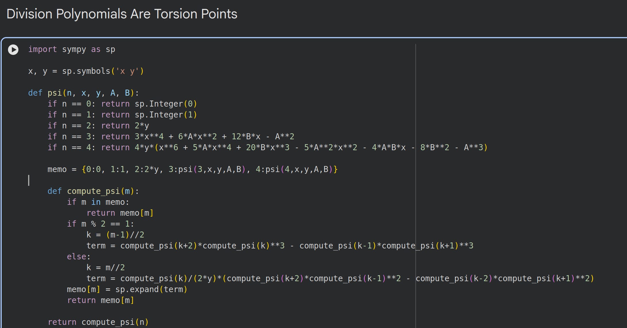
We first convert the division polynomial code from Part 4 into symbolic form using sympy:

Symbolic division polynomial in Python

We can verify our implementation using this example (Dinges, 2010):

The roots of our division polynomial shoul match this

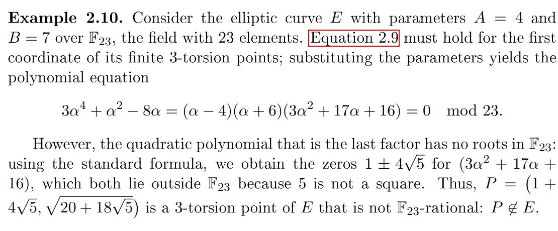
In Python, the example resembles:

Roots of symbolic division polynomial

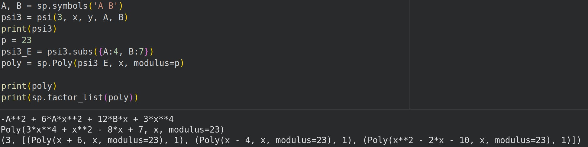
2.2 Frobenius Endomorphism

The Frobenius endomorphism is a mathematical shortcut for finding equivalent points on an elliptic curve by exponentiation. We’ll encounter this formal description in part 6:

Frobenius endomorphism. Taken from GLV paper in part 6

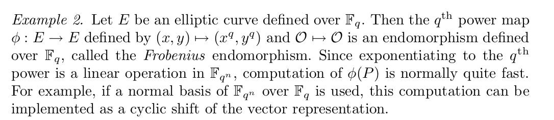
In part 2 we defined the trace of frobenius as the difference between predicted count of points and actual number of points on an elliptic curve in a finite field.

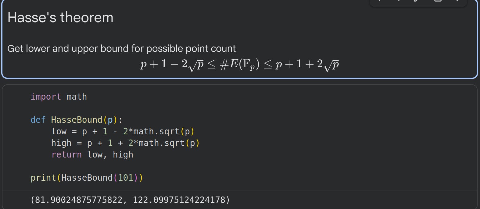
Hasse’s theorem relates the trace of frobenius to the number of points on an elliptic curve as given in (Lynn, 2025)⁴:

Hasse’s theorem. Taken from (Lynn, 2025)

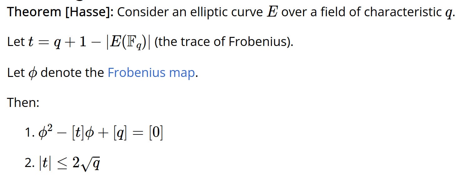
Hasse’s theorem bounds the possible number of points and Python code resembles:

Hasse's theorem in Python

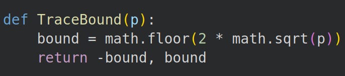
However, our goal is to bound the trace of frobenius and this resembles:

Bounding trace of frobenius in Python

Schoof’s algorithm demands us loop over small values of t in the characteristic equation until we find the one that satisfies:

We test the characteristic equation modulo small primes

2.3 Tying Everything Together

(Visser, 2020)⁵ summarizes the exact computation performed for Schoof’s algorithm:

Note: a is used in place of t to represent the trace of frobenius

Schoof’s algorithm. Taken from (Visser, 2020)

Where the sub-algorithm in Step 2 is:

Sub-algorithm. Taken from (Visser, 2020)

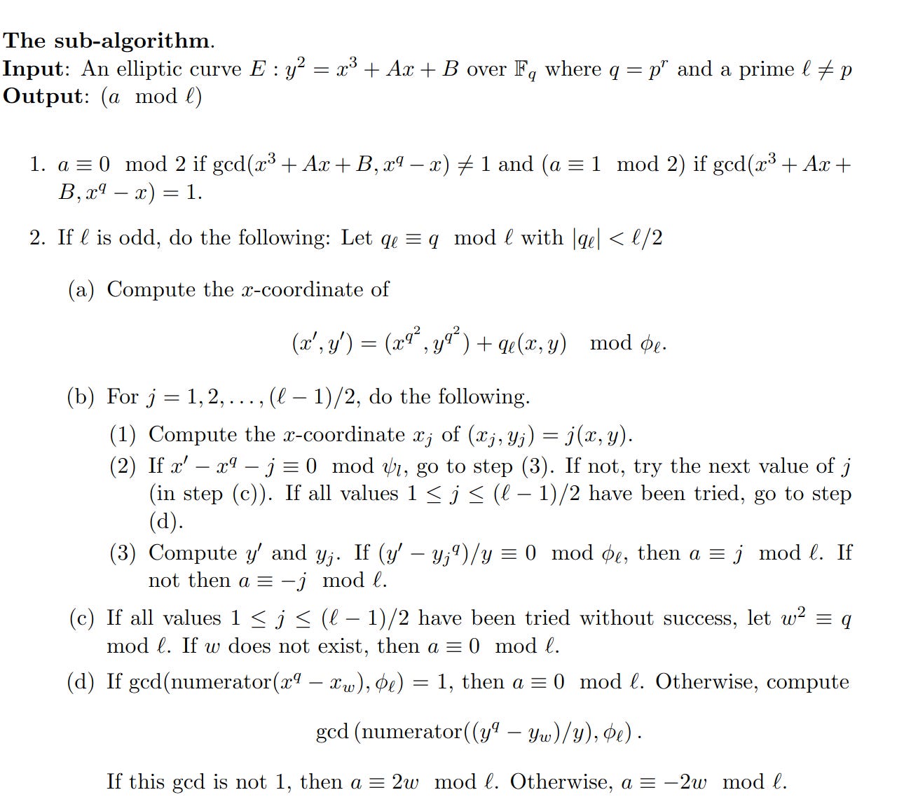
Note that field operations occur in the quotient ring highlighted below (Costello, )⁶:

Polynomial quotient ring needed for small odd primes. Taken from (Costello, 2020)

2.4 Final Python Code

Sympy can’t construct multivariate quotient rings (Sympy issue #20608, 2020)⁷.

This we overcome by finding a factor of the division polynomial (they tend to be reducible) then ‘lifting’ our curve to the field extension where the corresponding x-coordinate exists.

Let’s write some quick field extension arithmetic functions:

Arithmetic in a field extension

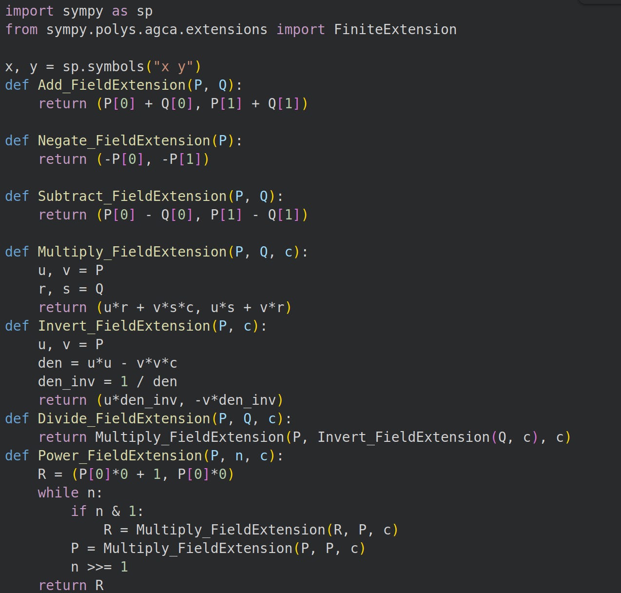
Next, we write scalar multiplication and the frobenius endomorphism that’s aware of the field extension:

Point addition, scalar multiplication and Frobenius endomorphism

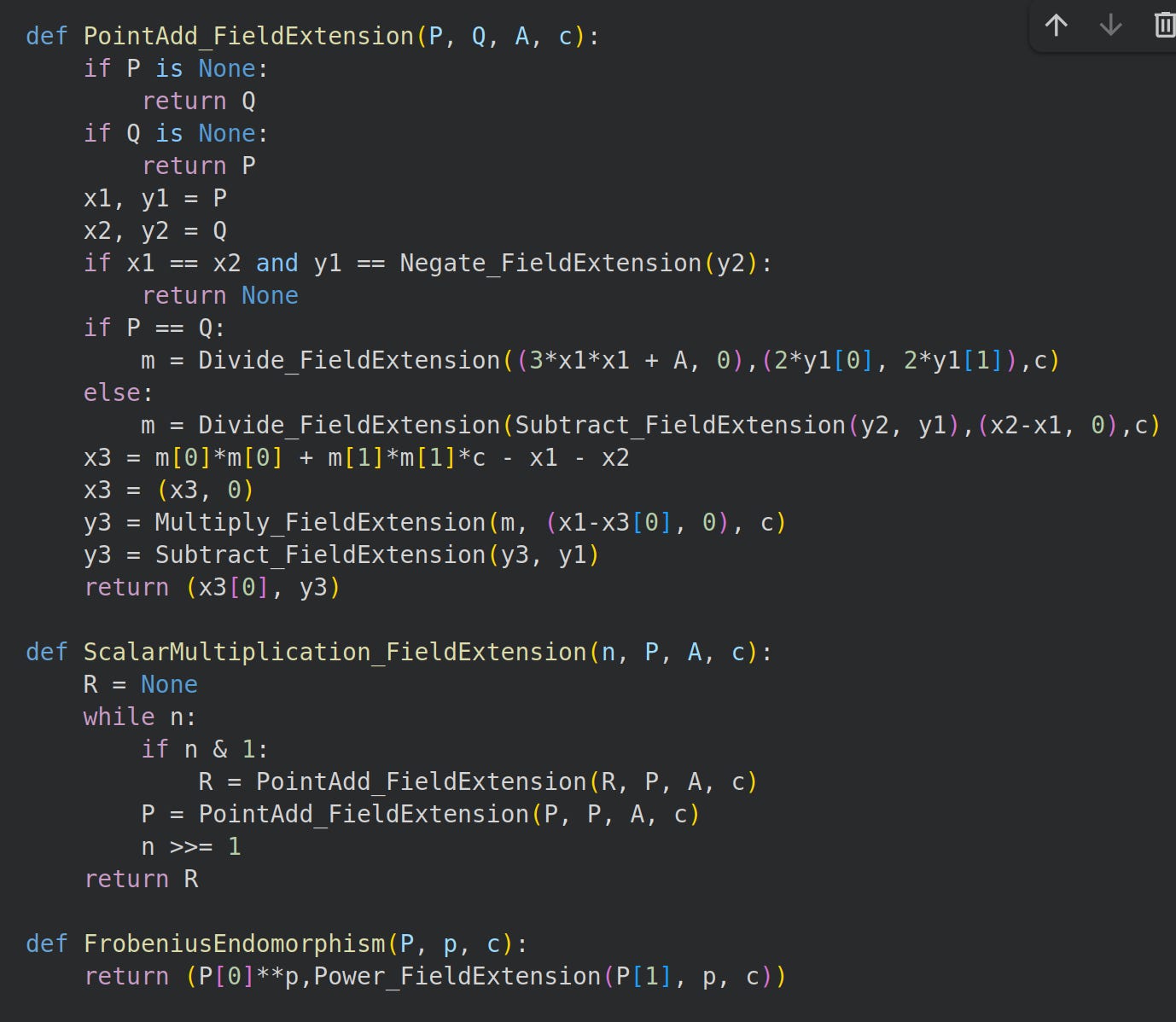
Now, we find the trace of frobenius modulo 2:

Trace modulo 2

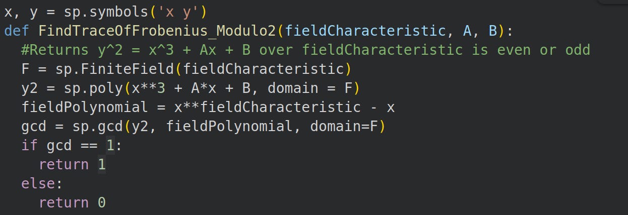
Next, we compute the trace of frobenius modulo small primes.

Trace modulo ell

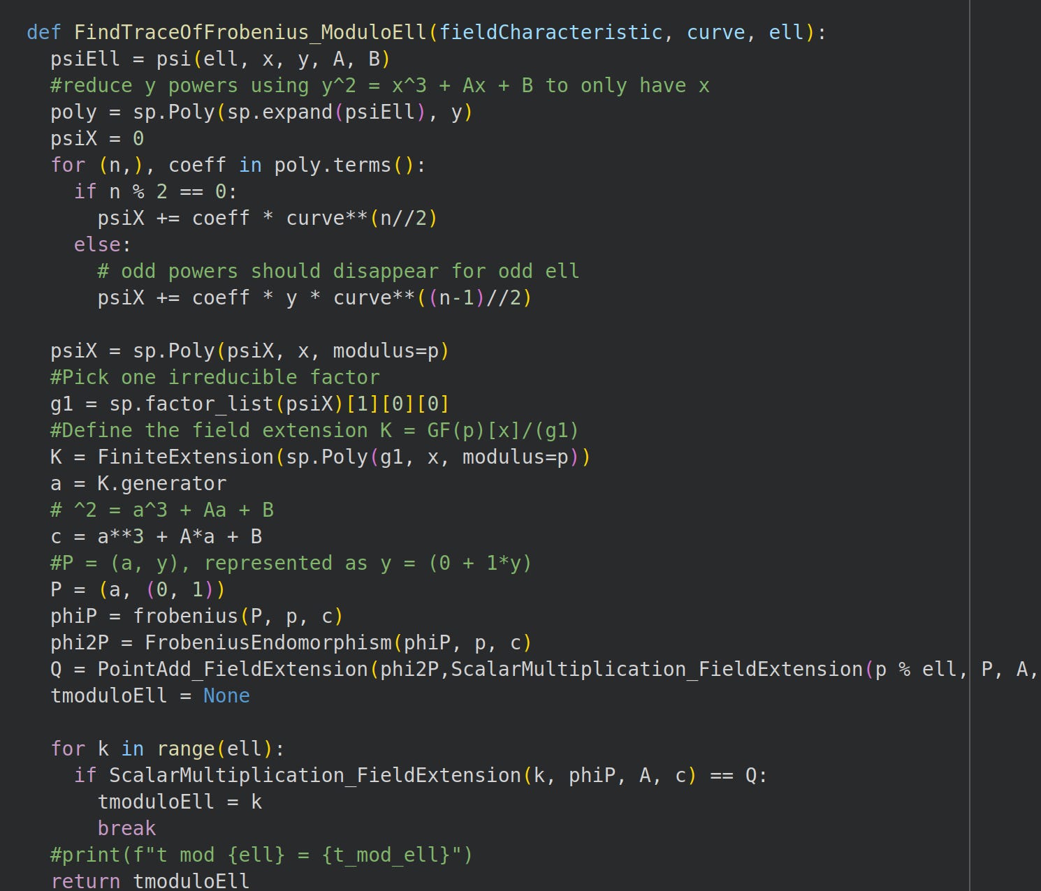
Let’s try our code on this Sage example:

Small elliptic curve where trace of frobenius is -6

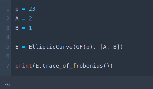
In the example above, we expect to see -6 modulo different small primes.

In Python, this resembles:

Predicted trace modulo small prime matches expected

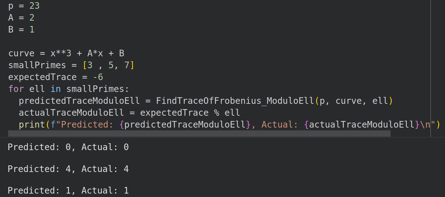
It works!

3.0 Recommended Reading

If you’ve never seen field extensions then you’d benefit from:

Commutative Complex Number Theory in Plain C

References

1. Schoof, R. (1985). Elliptic Curves over Finite Fields and the Computation of Square Roots mod p. Mathematics of Computation 44, no. 170 (1985): 483–94. PDF.

2. Sutherland, A. (2025). Elliptic Curves: Lecture 8 (Schoof’s Algorithm). MIT 18.783 Fall 2025. PDF.

3. Dinges, P. (2010). An Elementary Derivation and Implementation of Schoof’s Algorithm for Counting Points on Elliptic Curves. PDF. GitHub.

4. Lynn, B,. (2025). Counting Points. Link.

5. Visser, J. (2020). Schoof’s algorithm: Point counting on elliptic curves. University of Groningen. PDF.

6. Costello, C. (2026). Pairings for Beginners. PDF.

7. Benjamin, O. (2020). Multivariate Polynomial Quotient Rings. Issue number 20608. GitHub.